Introduction to GIS
Overview course content
Introduction to GIS
| 1 | Basics of GIS | 2 |
| 2 | Spatial data | 4 |
| 3 | Spatial reference systems | 3 |
| 4 | Spatial data basic analysis | 3 |
| 5 | Data visualization | 2 |
Overview course content
Introduction to GIS
Learning outcomes:
- Understand the basic concepts of Geographic Information Systems
- Define terms related to raster and vector data models
- Compare vector and raster data models
- Understand the difference between geographic and projected coordinate systems
- Select spatial objects using attribute and spatial queries
- Perform simple analysis with geoprocessing tools
- List map elements and basic principles of map creation
- Create a thematic map using different methods of symbolization
1 | Basics of GIS
Introduction to GIS
| # | Content |
| 1.1 | What is GIS? |
| 1.2 | Uses of GIS |
1.1 | What is GIS?
GIS definition
Geographic Information System (GIS)
"is a computer system capable of capturing, storing, analyzing, and displaying geographically referenced information; that is, data identified according to location. Practitioners also define a GIS as including the procedures, operating personnel, and spatial data that go into the system."
"is a computer-based tool for mapping and analyzing things that exist and events that happen on earth. GIS technology integrates common database operations such as query and statistical analysis with the unique visualization and geographic analysis benefits offered by maps."
The spatial (geographic) part differentiates a GIS from a standard computer database.
GIS components
A GIS consists of five key components: hardware, software, data, people, and methods.
 |
 |
 |
 |
 |
GIS: main idea
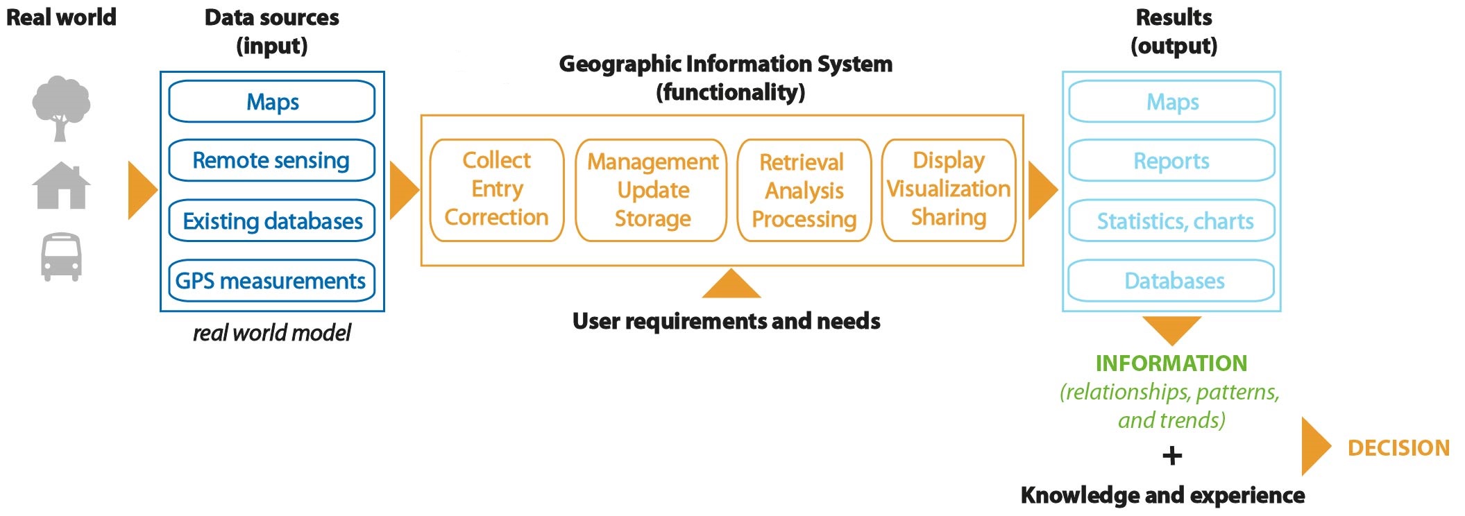
The main goal of GIS is to provide spatial information to decision makers.
Data vs. Information
Data means simply facts or figures - pieces of information, but not information itself.
Data is collected and stored in databases. When data are processed, interpreted, organized, structured or presented so as to make them meaningful or useful, they are called information. Information provides context for data.
In a GIS, spatial analysis and modelling are the main source of information.
Spatial analysis - a set of methods and tools for performing operations on spatial data in order to obtain additional information.
1.2 | Uses of GIS
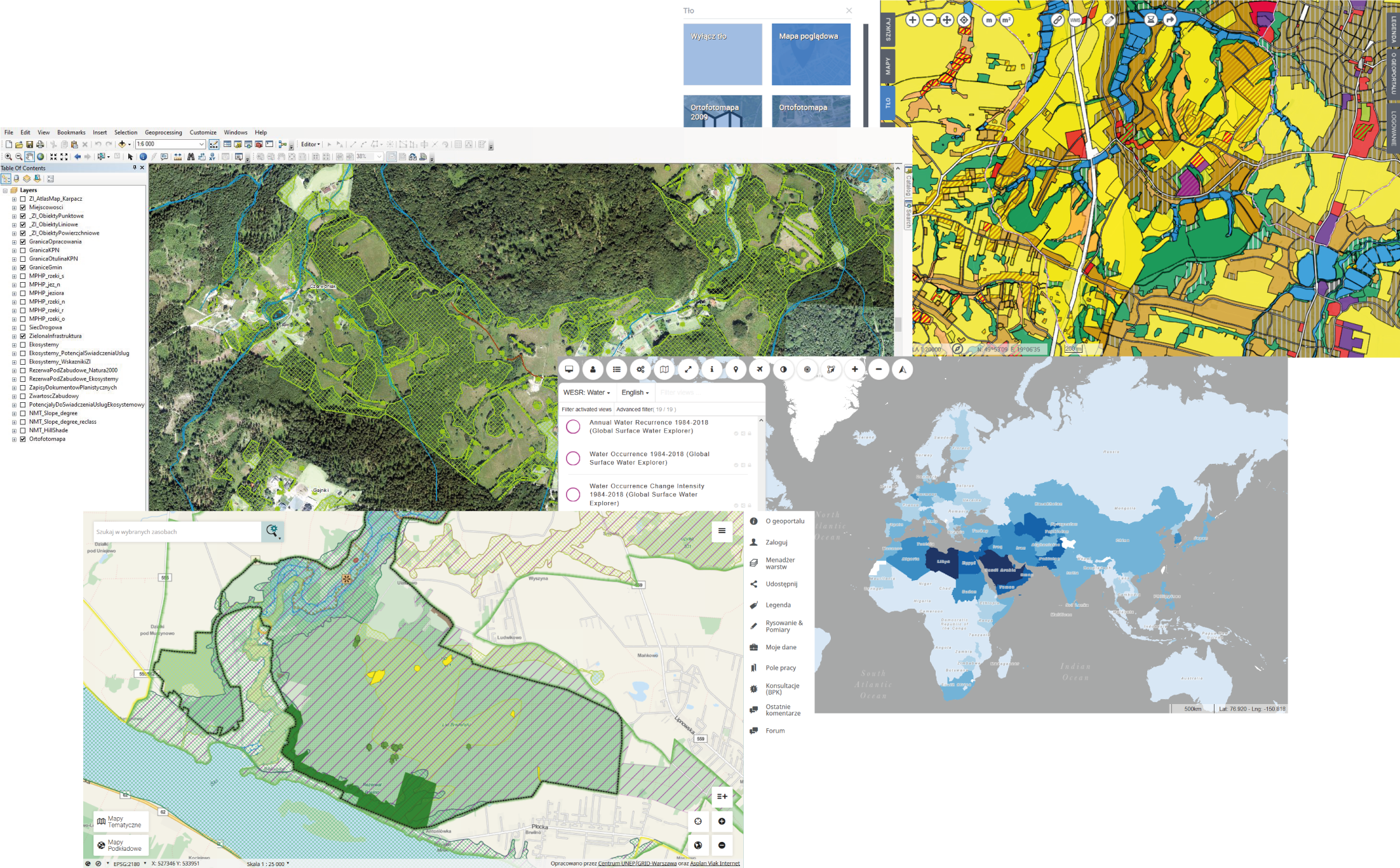
Software
Geospatial software and tools:
- Desktop GIS (QGIS, SAGA GIS, GRASS GIS, ILWIS, IDRISI, Esri products: ArcGIS, ArcMap, ArcGlobe, GeoMedia, MapInfo, Bentley Systems: MicroStation, ENVI, ERDAS IMAGINE)
- GIS as a service (ArcGIS Online, Mapbox, OpenStreetMap, Google Maps, Apple Maps, Here Maps, Bing Maps)
- Spatial database management systems (MySQL, Oracle Spatial, Microsoft SQL Server, PostgreSQL)
- Map servers (Geoserver, MapServer, Mapnik)
|
|
 |
Fields of GIS usage
 |
|
Advantages of GIS
- Ability to view, visualize and interpret data in the form of maps, charts and reports - relationhips and trends easy to see and understand
- Improved decision making and problems solving through specific and detailed information regarding locations of features and phenomena
- Reduce costs and increase efficiency
- Improved communication between organisations or departments
2 | Spatial data
Introduction to GIS
| # | Content |
| 2.1 | Definition and properties |
| 2.2 | Vector data model |
| 2.3 | Raster data model |
| 2.4 | Comparing vector and raster data models |
2.1 | Definition and properties
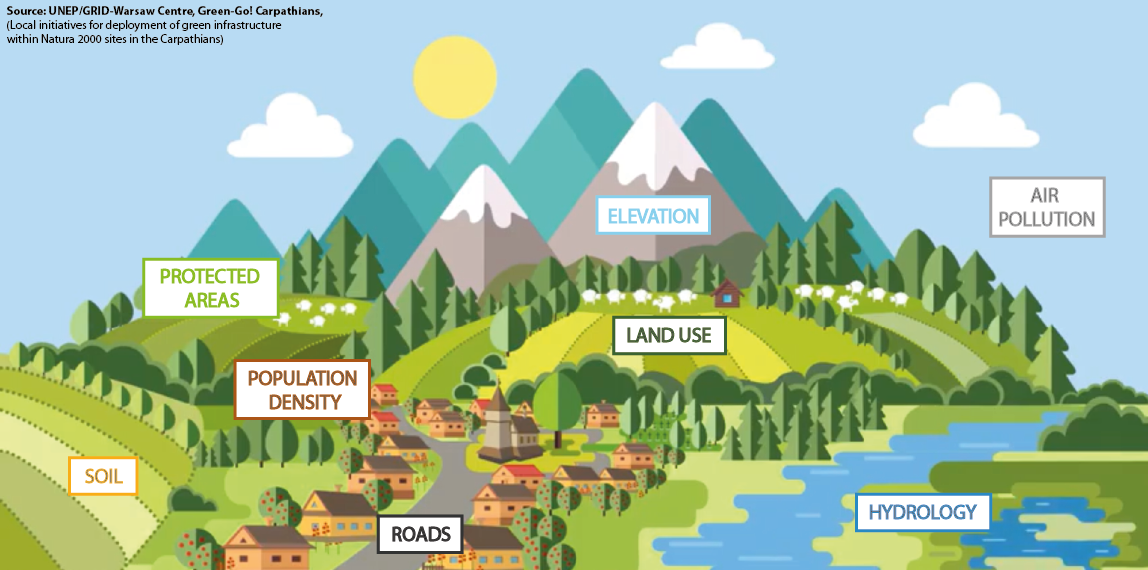
From real world...
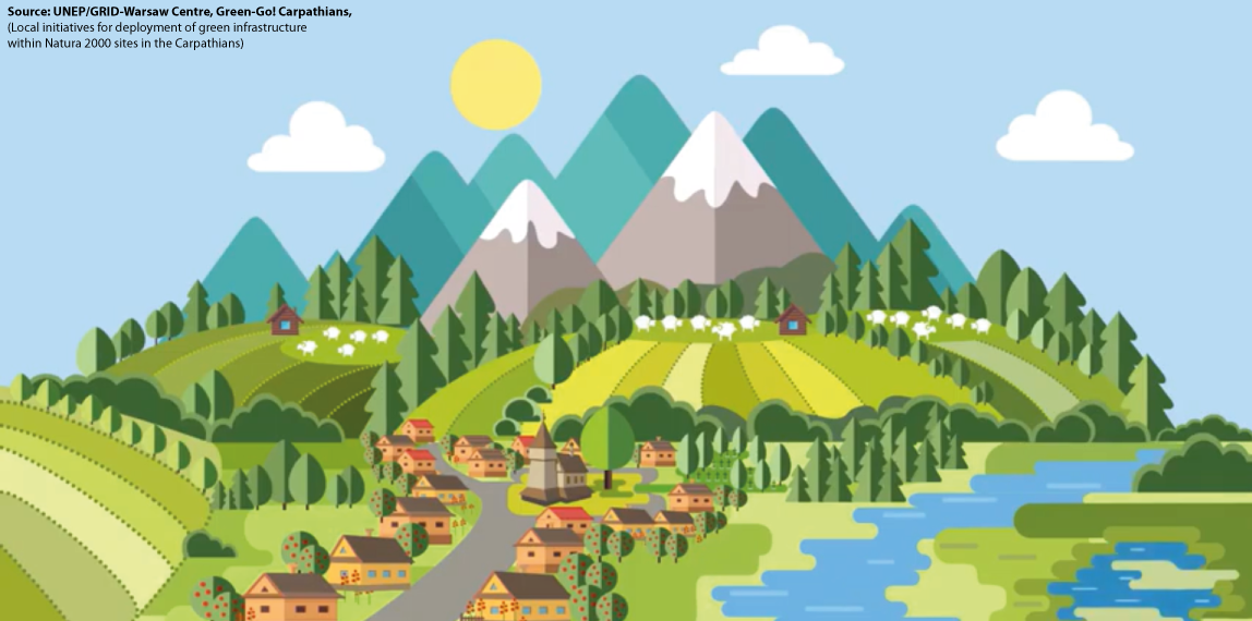
... to GIS
Spatial data - definition
Spatial object means an abstract representation of a real-world phenomenon related to a specific location or geographical area.
Spatial data means any data with a direct or indirect reference to a specific location or geographical area.
Spatial data set means an identifiable collection of spatial data.
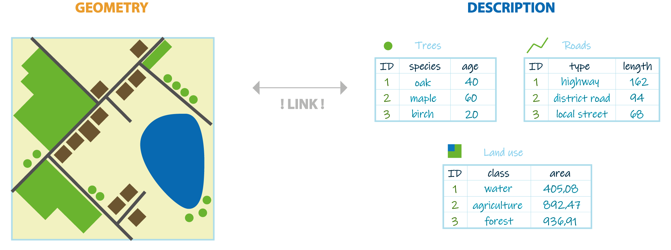
Data model
Data model is a set of guidelines to convert the real world (called entity) to the digitally and logically represented spatial objects consisting of the attributes and geometry.
The attributes are managed by thematic or semantic structure while the geometry is represented by geometric-topological structure.
Spatial data - properties
Spatial data describes shape, location, spatial relationships and attributes of features related to the Earth's surface.
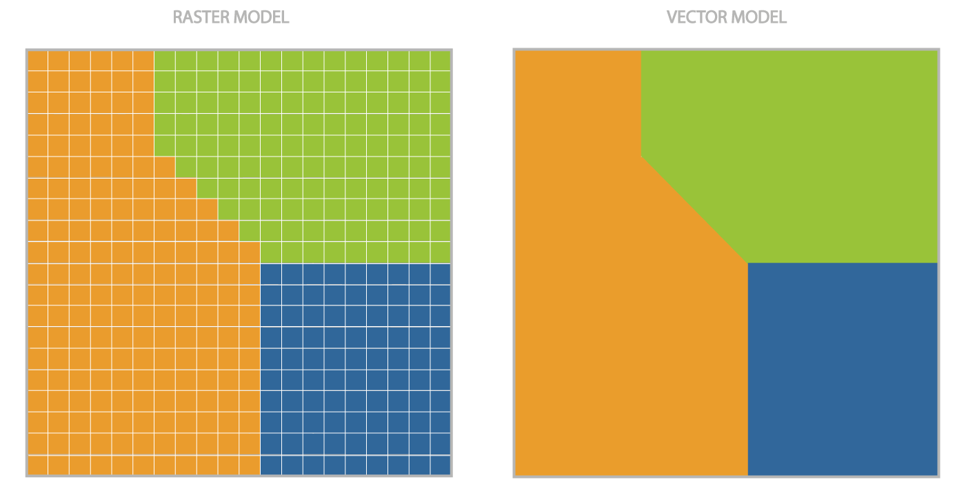
Spatial data (representation) model
Two common spatial data models:
VECTOR

RASTER

2.2 | Vector data model
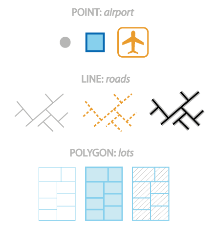
Three types of geometry
A vector data model defines discrete objects such as fire hydrants, rivers, lakes.
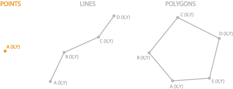
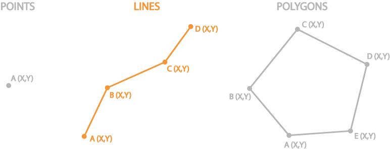
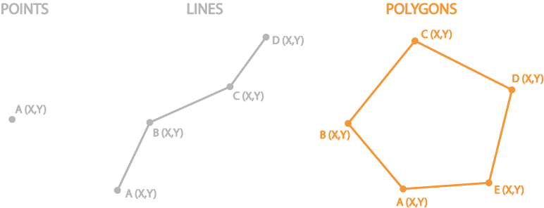
A vector data models divided into three basic types:
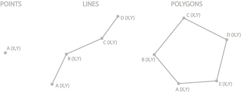
All three of these types of vector data are composed of coordinates and attributes attached to the geometry.
Geometry: points
 |
|
Geometry: lines
 |
|
Geometry: polygons
|
|
Geometry: spaghetti vs. topological model
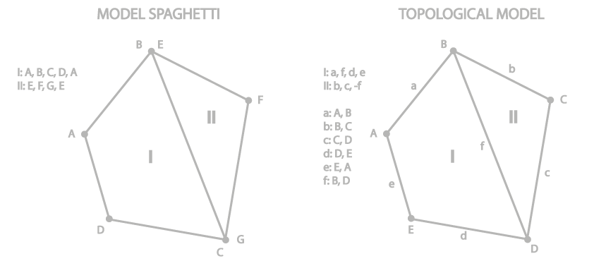
Topology
Topology is required to determine spatial relationships between objects in a GIS.
If the features are deformed (e.g. through projections or datum transformations), some properties change: area, shape, direction, distance, relative proximities.
Other properties (topological properties) remain constant after distortion: adjacency, containment, connectivity.
Benefits of topology:
- storing data more effeciently
- ensuring data quality
- facilitating advanced spatial analysis (e.g. network analysis)
Topology
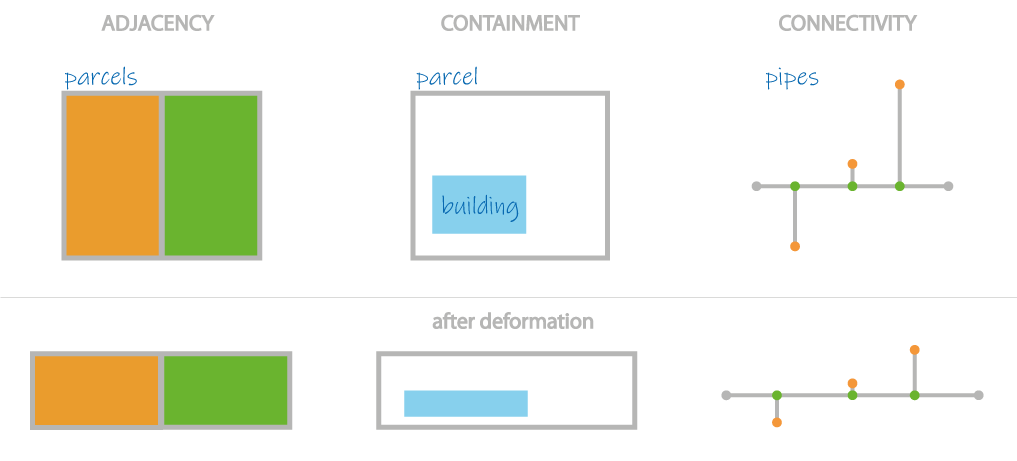
Three examples of properties that remain constant after deformation
Attribute table
|
An attribute is a nonspatial information about a geographic feature in a GIS, usually stored in a table and linked to the feature by a unique identifier (ID). A database or tabular file containing information about a set of geographic features, usually arranged so that:
The attribute values can be used to find, query, analyze and symbolize features. |
 |
Attribute table - data types
Each column in the database may contain different type of data.
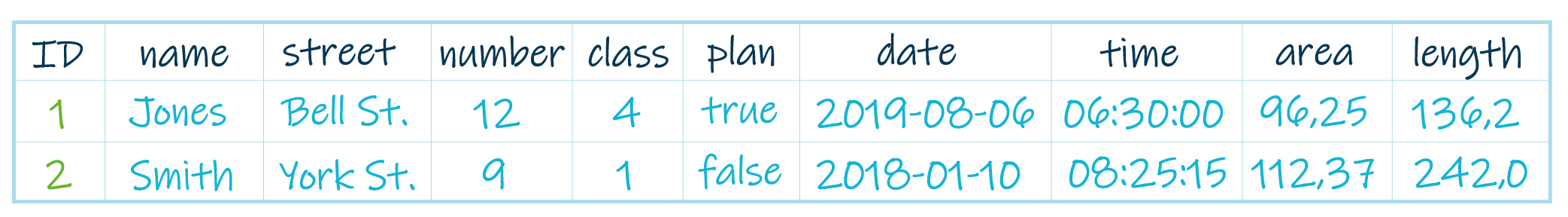
Basic data types:
- NUMERIC: INTEGER (long int, short int) - numbers, code list
- NUMERIC: FLOAT (double, real) - floating-point numbers
- STRING (char, varchar, text) - names and other texts
- DATE/TIME (date, time, year, timestamp) - data and/or time
- BOOLEAN (0/1, true/false, yes/no) - logical expression
- BLOB - multimedia files
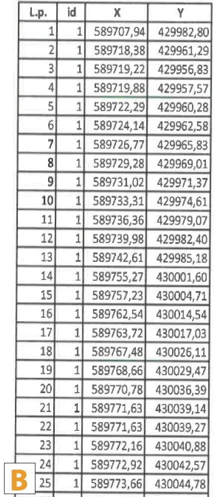
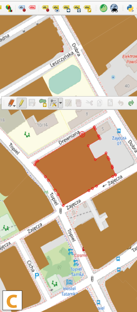
Vector data sources
 |
 |
 |
 |
 |
Vector data sources
(A - GPS measurements, B - list of coordinates, C - digitizing and conversion tools e.g. raster to vector, D, E - existing databases)
Vector file formats
- ESRI Shapefile - the most common geospatial file type developed by ESRI, consists of:
- shp (feature geometry)
- shx (shape index position)
- dbf (attribute data)
- prj (projection system metadata)
- xml (associated metadata)
- GML (Geography Markup Language) - XML based open standard for GIS data exchange
- KML/KMZ (Google Keyhole Markup Language) - XML based open standard for GIS data exchange
- GPX (GPS eXchange Format) - GPS data file
- GeoJSON (Geographic JavaScript Object Notation) - a lightweight format based on JSON, used by many open source GIS packages
2.3 | Raster data model
Raster data model
A raster data model defines continous data and phenomena.
Raster's are:
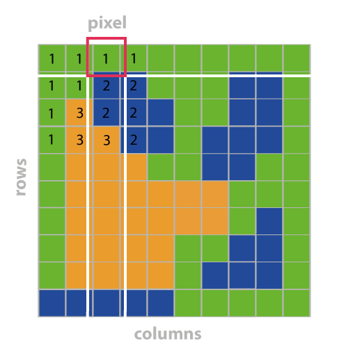
Raster data model: geometry
A raster consists of a matrix of cells (or pixels) organized into rows and columns (or a grid) where each cell contains one value representing information such as temperature, elevation, or spectral data. Pixel - smallest visible element of an image. Grid - 2-D object feature that represents a single element of a continous surface. |
 |
Raster data model: georeferencing
Cells are identified by their positions in the grid. Raster data is georeferenced by: |
|
Spatial resolution
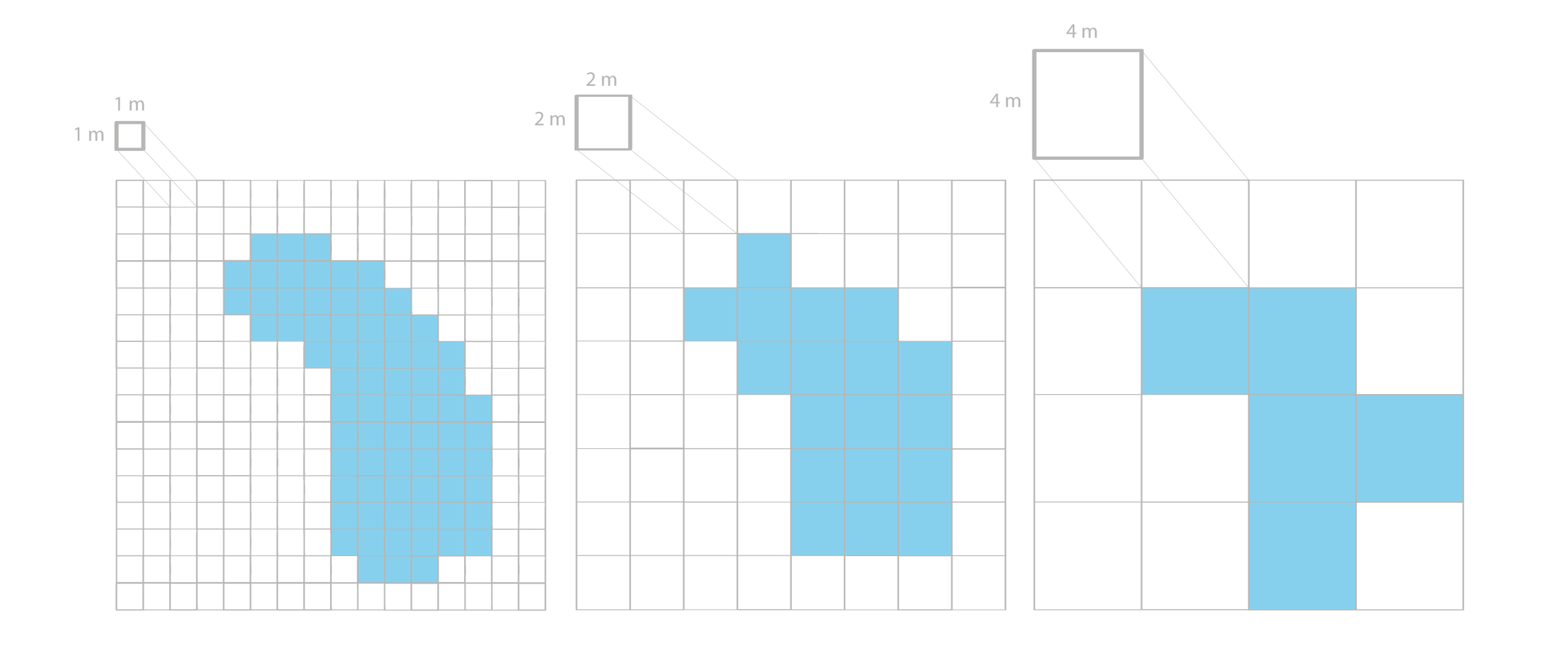 The same feature in images of different resolution
A spatial resolution refers to the dimension of the cell size representing the area covered on the ground. Higher resolution means better feature quality but it means also bigger raster file size.
Raster bands
A raster dataset contains one or more layers called bands.
A band is represented by a single matrix of cell values.
For example, a digital elevation model (DEM) is a single-band raster (has one band holding elevation values) while satellite imagery is a multispectral image and has multiple bands.
Three main ways to display single-band raster datasets:
Raster bands
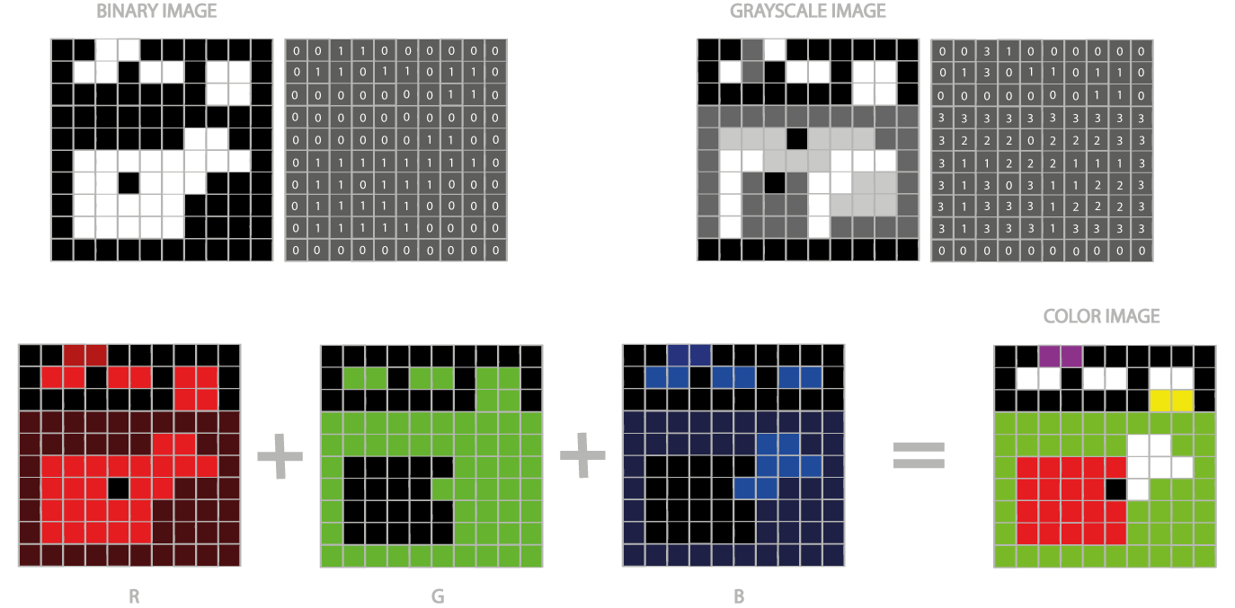
Three ways to display raster dataset (binary image, grayscale image and color image)
Attribute table
Raster data can also have attributes only if pixels are represented using a small set of unique integer values. Raster datasets that contain attribute tables typically have cell values that represent or define a class, group, category, or membership.
In raster datasets, each row of an attribute table corresponds to a certain zone of cells having the same value.
The attribute tables can be used to analyze datasets and symbolize raster cells.
Note: Not all GIS raster data formats can store attribute information.
Attribute table
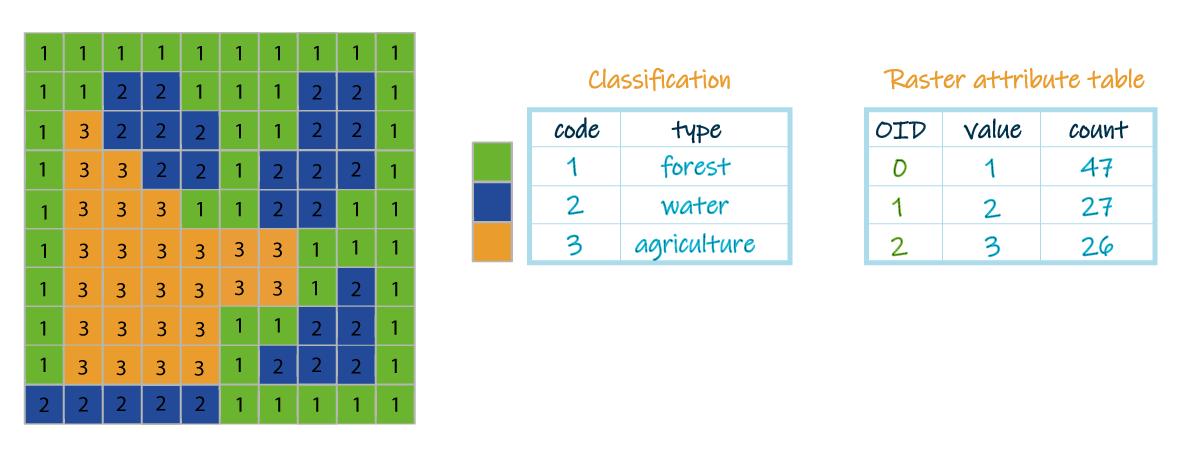
An example of raster dataset with attribute table
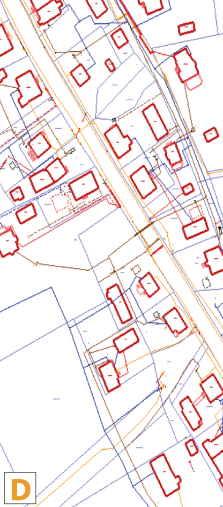
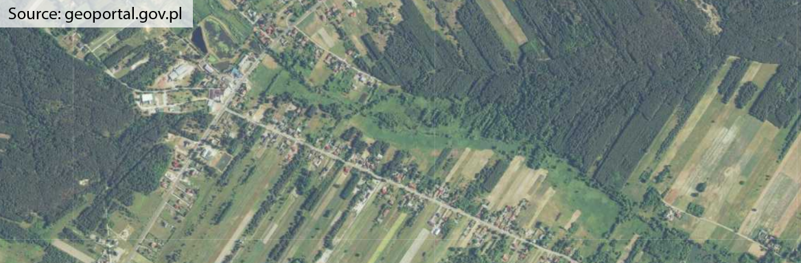
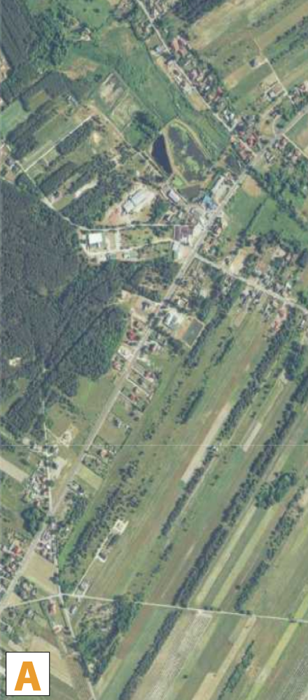
Raster data sources
 |
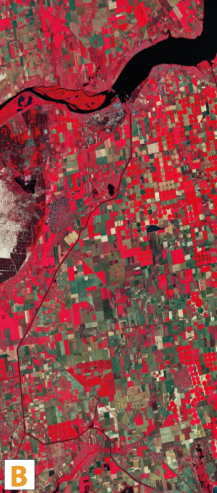 |
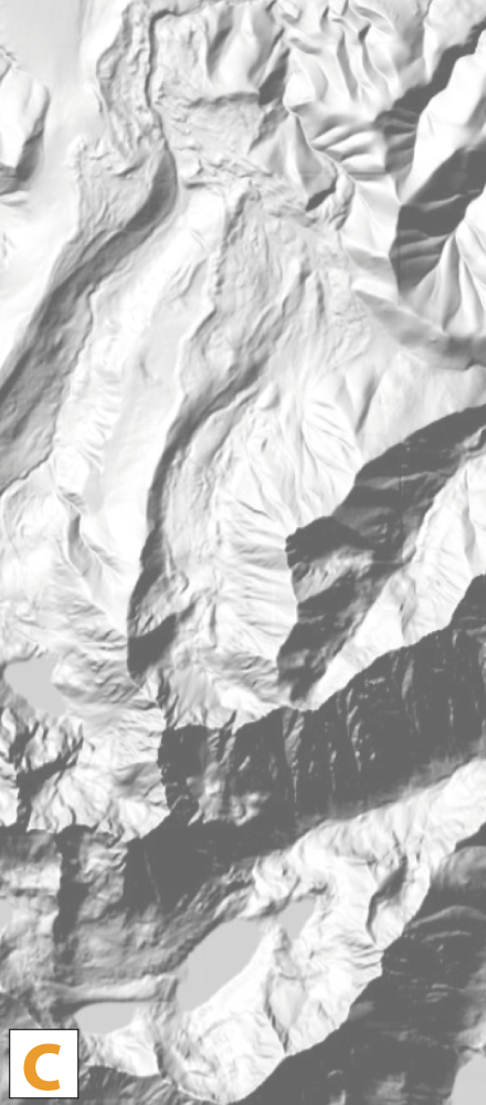 |
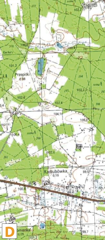 |
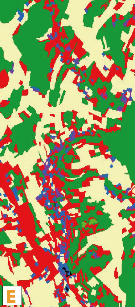 |
(A - orthophoto, B - satellite imagery, C - DEM, D - scanned maps and plans, E - conversion and analysis tools e.g. vector to raster, interpolation)
Raster file formats
- GeoTIFF - TIFF variant enriched with GIS relevant metadata, may be accompanied by other files:
- tfw (raster geolocation)
- xml (metadata)
- aux (projections and other information)
- ovr (pyramid files improves performance for raster display)
- IMG - ERDAS IMAGINE image file format
- ESRI Grid - format developed by Esri, which has two varieties: binary or ASCII
2.4 | Comparing vector and raster data models
Comparing: vector vs. raster data model
| properties | vector | raster |
|---|---|---|
| depict | discrete features | continous data |
| geometry | coordinates | cells organized into a grid |
| attributes | attribute table (with many attributes) | cell value (only one attribute) |
| analysis | geoprocessing | map algebra, overlays |
| data structure | more complex | more simple |
| size | compact data structure – little storage space | greater storage needed |
| file formats | ESRI Shapefile, GML, KML, geoJSON, GPX | geoTIFF, IMG, grid |
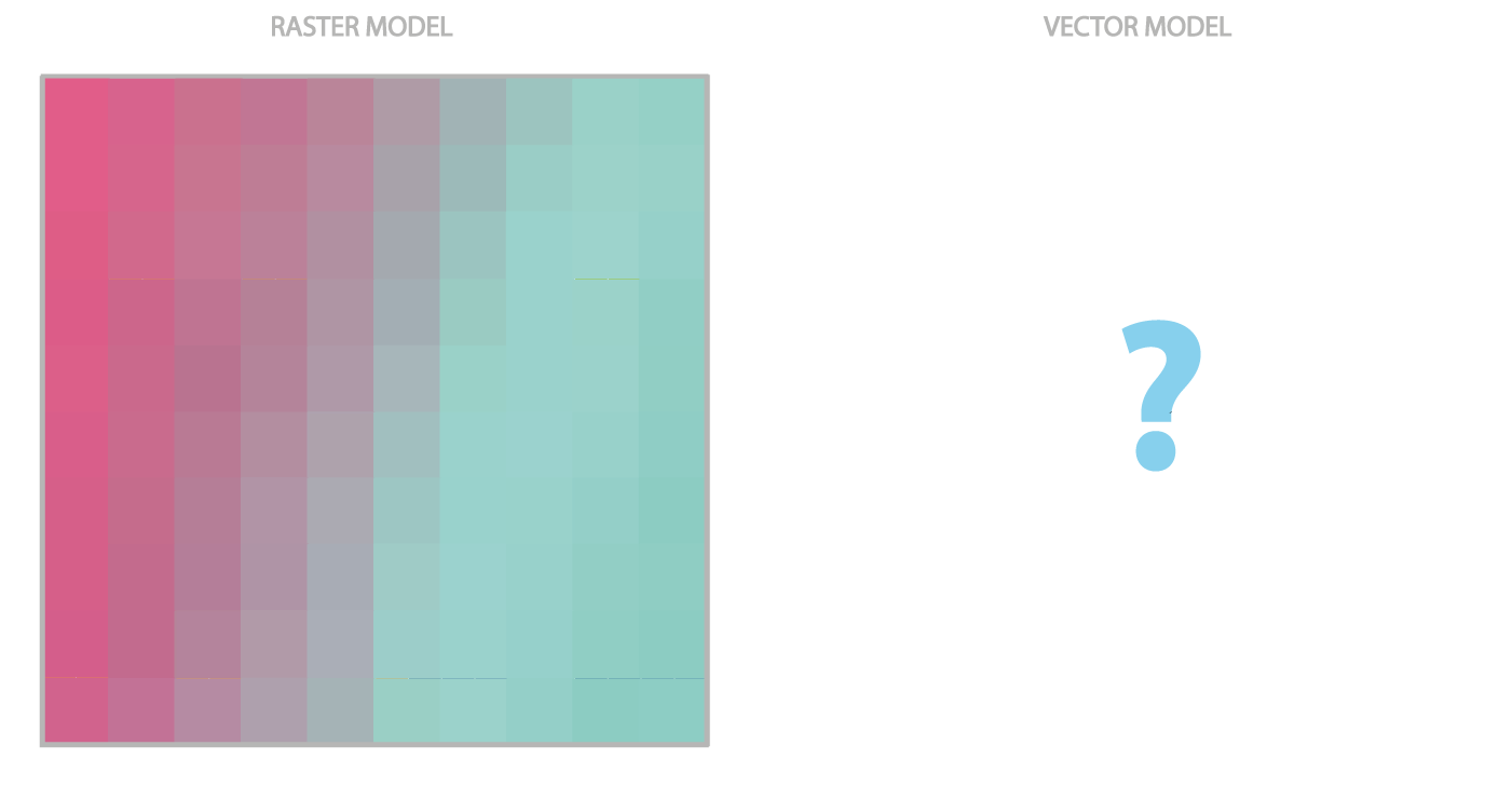
Which one is better?
Which one is better?
3 | Spatial reference systems
Introduction to GIS
| # | Content |
| 3.1 | Definition |
| 3.2 | Geographic Coordinate System |
| 3.3 | Projected Coordinate System |
3.1 | Definition
What is spatial reference?
A spatial reference describes where features are located in the real world. It is a key component of spatial data and applications, and differentiates a GIS from a standard databases.
A spatial reference system (SRS) or coordinate reference system (CRS) is a coordinate-based local, regional or global system used to locate geographical entities.
Eiffel Tower - where is it?
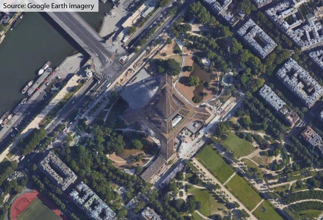
Champ de Mars, 5 Avenue Anatole France, 75007 Paris, France
48° 51' 29.1348''N; 2° 17' 40.8984''E = 48.858093; 2.294694
448256.00 m E; 5411928.00 m N
Types of coordinate systems used in a GIS
Two common types of coordinate systems used in a GIS:
Coordinate systems (both geographic and projected) provide a framework for defining real-world locations.
3.2 | Geographic Coordinate System
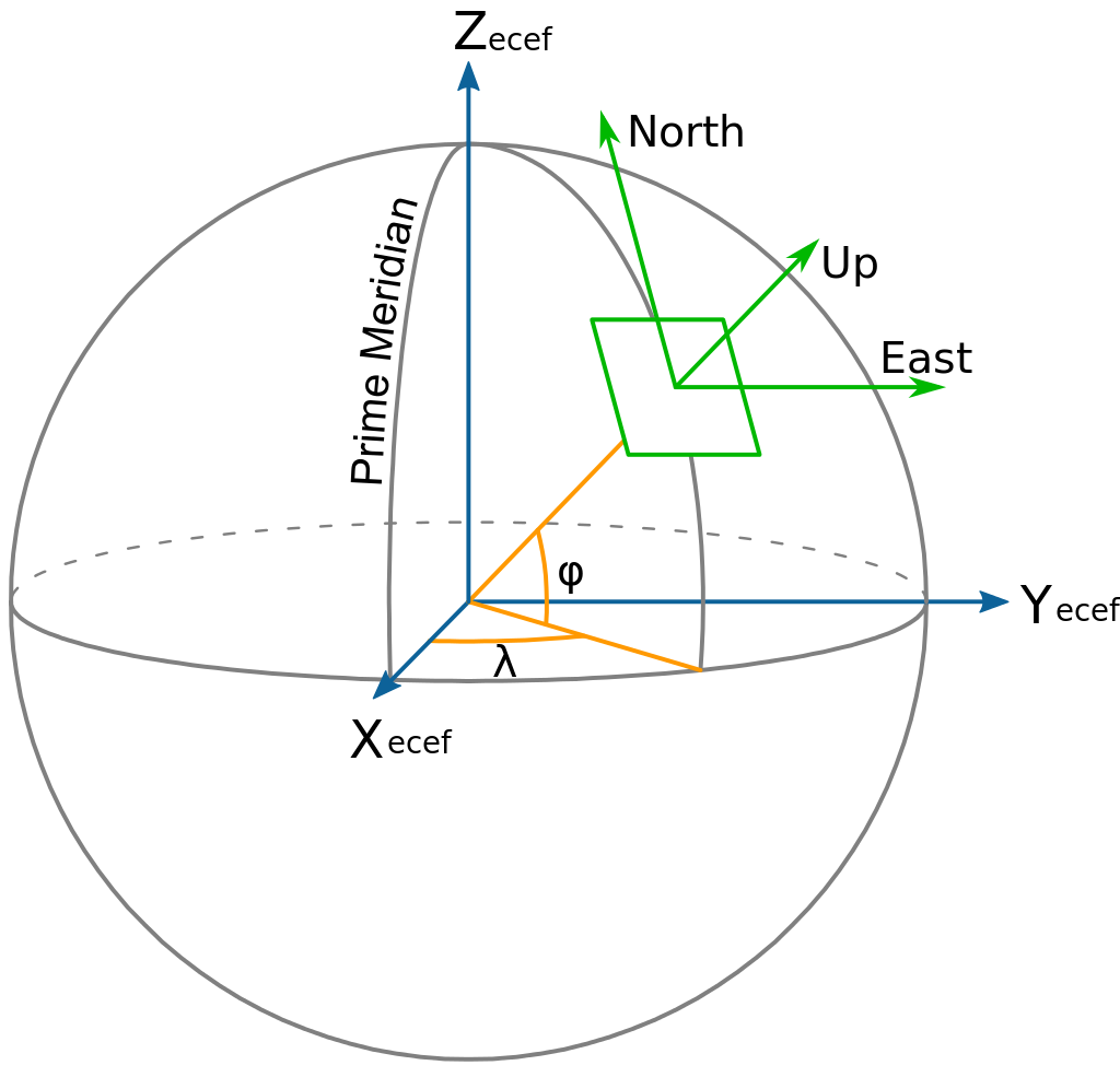
Geographic Coordinate System
A geographic coordinate system is a reference system for identifying locations on the curved surface of the earth. Locations on the earth’s surface are measured in angular units from the center of the earth relative to two planes: the plane defined by the equator and the plane defined by the prime meridian (which crosses Greenwich England). A location is therefore defined by two values: a latitudinal value and a longitudinal value.
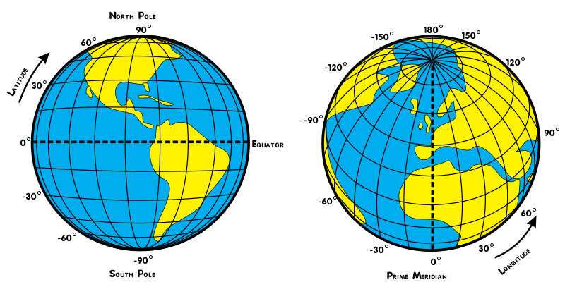
Latitude and Longitude (Wikimedia Commons)
Geographic Coordinate System
|
Latitude and Longitude - relationships
|
Geographic Coordinate Systems can only be used to measure angles, not distances or areas.
3.3 | Projected Coordinate System
Projection
Projection is a method by which the curved surface of the Earth is portrayed on a flat surface. This requires a systematic mathematical transformation of the Earth’s graticule of lines of longitude and latitude onto a plane. All projection types can be aggregated into three groups: planar, cylindrical and conical.
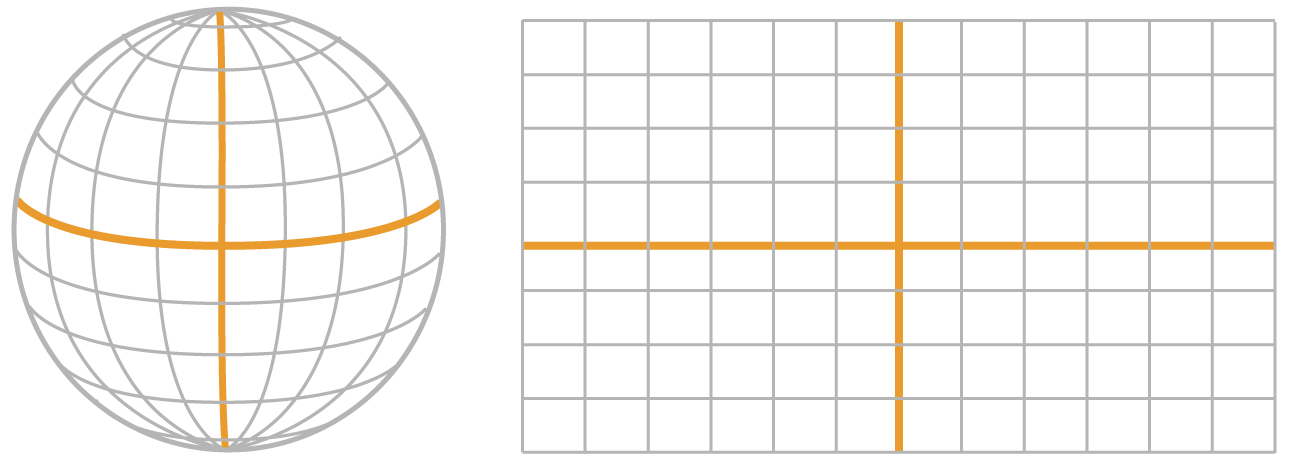
The idea of projection - mapping the Earth on a flat surface
In a projected coordinate system, locations are identified by X, Y coordinates on a grid.
Unlike a geographic coordinate system, a projected coordinate system can be used to measure distances and areas.
Planar projection
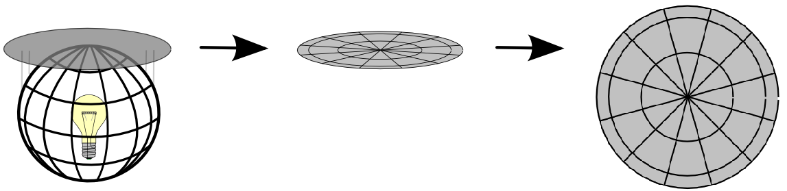
A planar projection maps the Earth's surface to a flat surface (QGIS Documentation)
Planar projection types
Planar projections can be of three different types:
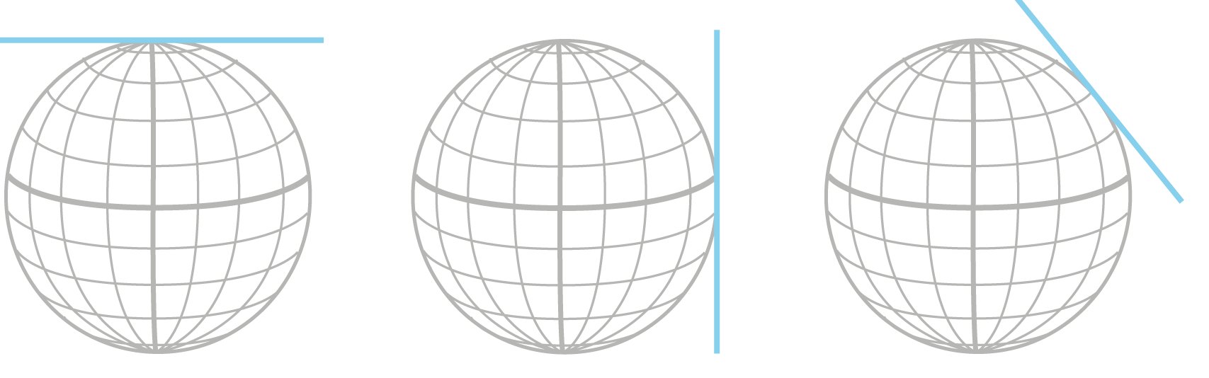
Three different types of planar projection (polar, equatorial, oblique)
Cylindrical projection
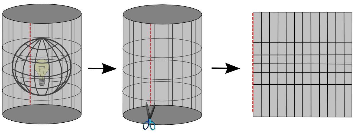
A cylindrical projection maps the Earth's surface to a flat surface (QGIS Documentation)
Conical projection
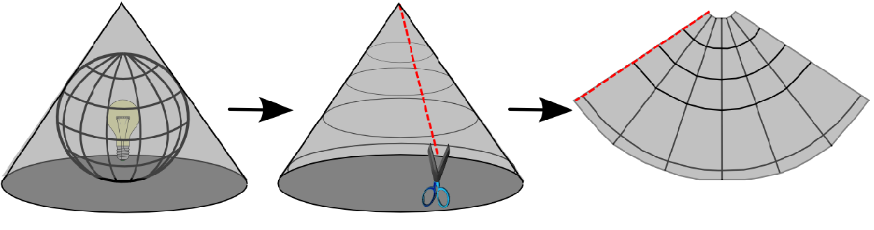
A conical projection maps the Earth's surface to a flat surface (QGIS Documentation)
EPSG code
The EPSG codes are 4-5 digit numbers that represent coordinate reference system definitions.
Most geographic information systems use EPSG codes as Spatial Reference System Identifiers (SRIDs) and EPSG definition data for identifying projections and performing transformations between these systems.
Common EPSG codes:
- EPSG:4258 - ETRS89 (European Terrestrial Reference System 1989), geodetic coordinate system for Europe
- EPSG:4326 - WGS 84, latitude/longitude coordinate system based on the Earth's center of mass, used by the Global Positioning System among others
- EPSG:3857 - Web Mercator projection used for display by many web-based mapping tools, including Google Maps and OpenStreetMap
4 | Basic analysis of spatial data
Introduction to GIS
| # | Content |
| 4.1 | Attribute query |
| 4.2 | Spatial query |
| 4.3 | Geoprocessing |
4.1 | Attribute query
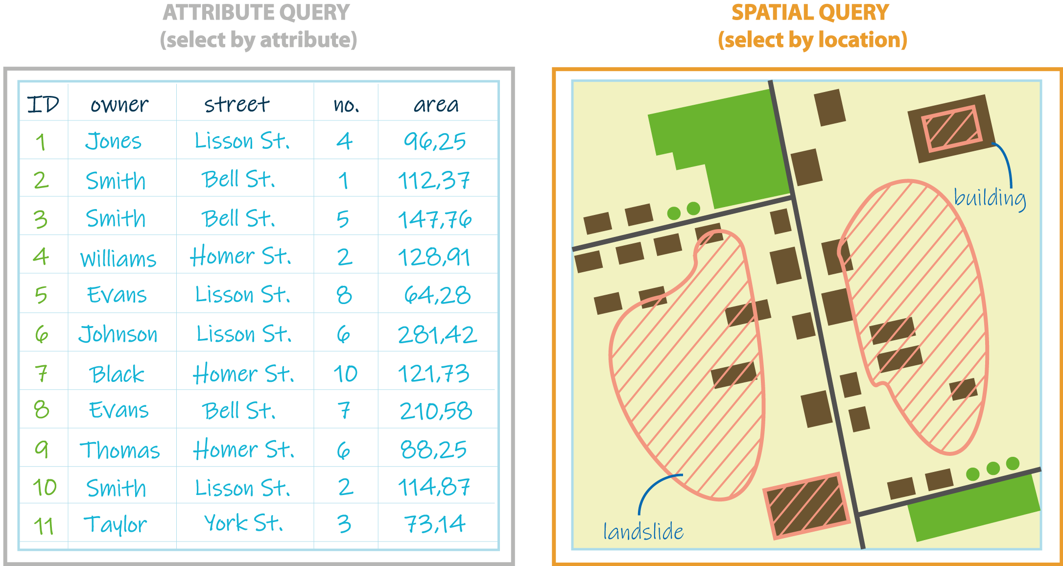
Attribute query - definition
Query is a request to select features or records from a database. Often written as a statement or logical expression.
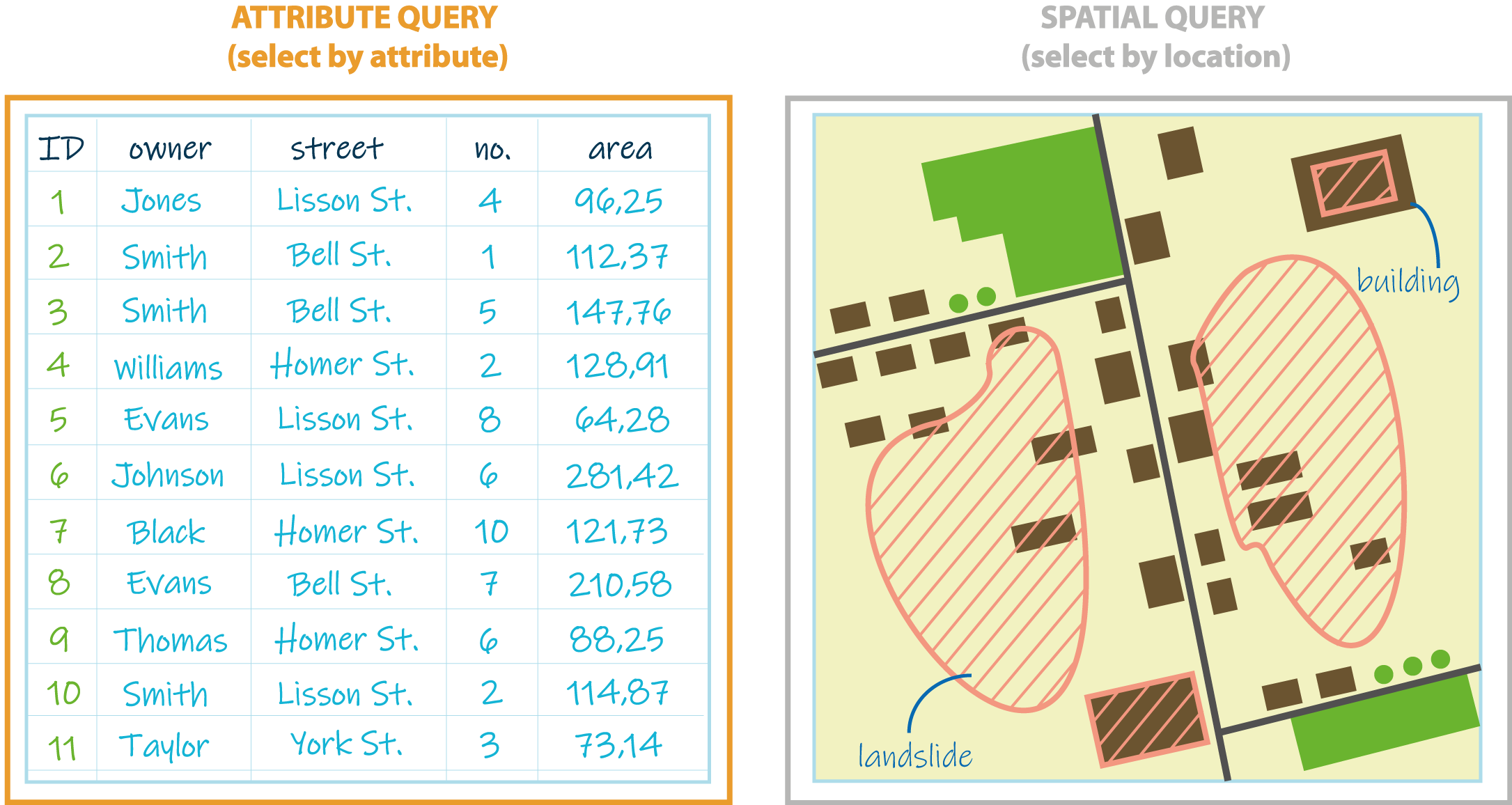
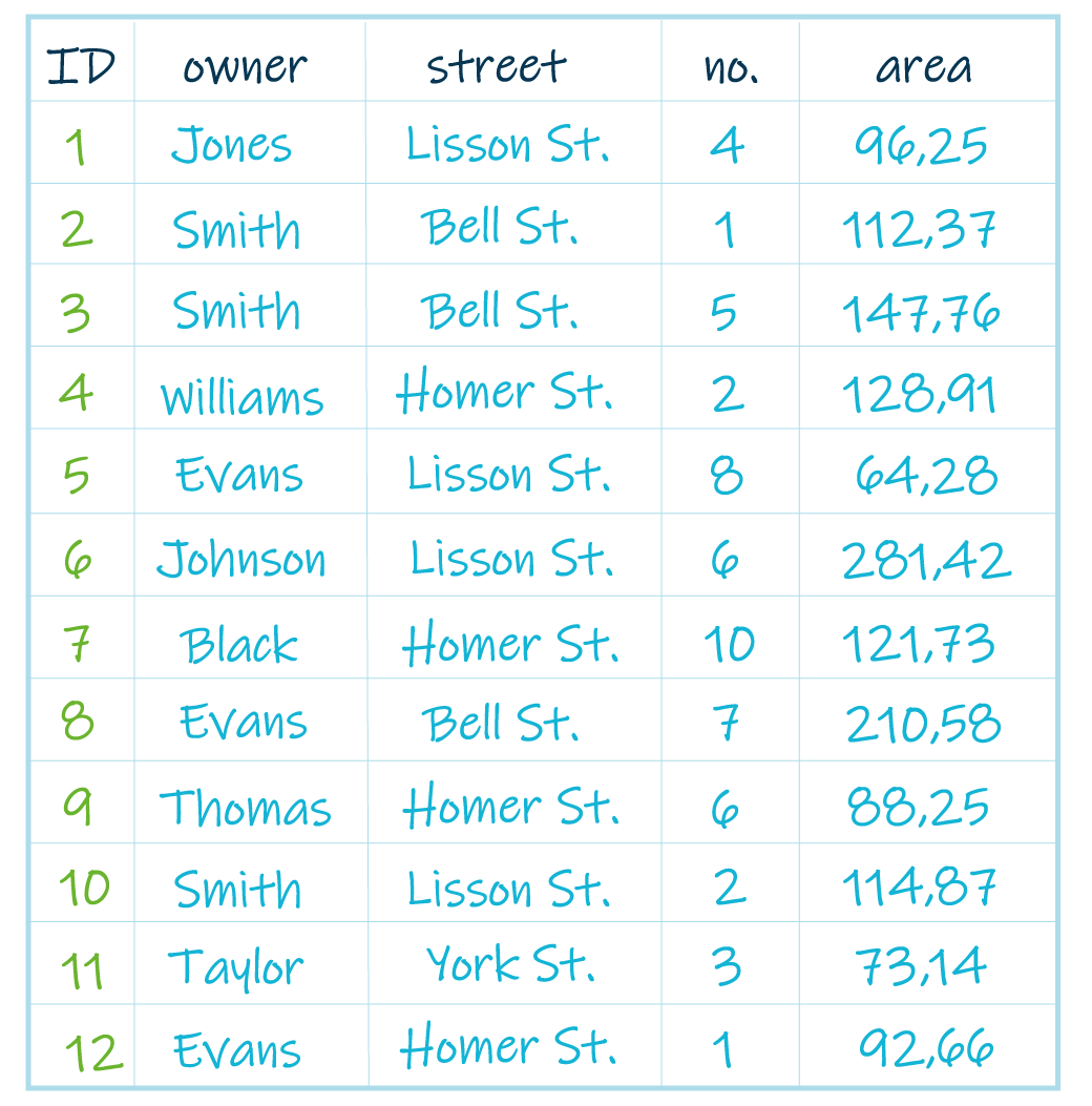
Attribute query is the process of searching and retrieving records of features in a database based on desired attribute values.
Attribute query
Typically, attribute query is performed using a criteria-based query language, most commonly SQL.
SQL (eng. Structured Query Language) is a domain-specific language used in programming and designed for managing data held in a relational database management system (RDBMS).
In most cases, the desired information can be given as a set of criteria based on the available attributes. These criteria are formatted in the appropriate query language as a Boolean expression, which can be validated as either true or false for each record in the database.
Individual criteria can be constructed and combined using:
- logical operators such as comparisons (>, <, =, >=, <=),
- Boolean algebra (and, or, not),
- functions (sin, cos, sqrt, etc.).
Where? How many? Which one? Whose?
 |
|
How to create an attribute query?
An attribute query consists of three basic elements: attribute field, operator, and attribute value.
1 element of the query is ALWAYS:
SELECT * FROM "name of field" WHERE operator 'value'
Examples:
Several elements of the query can be combined with operators: OR and AND.
Simple queries - operators
LIKE - search for a specified pattern in a column
BETWEEN ... AND ... - select values within a given range (concerns numbers, text, or dates)
IN (..., ...) - specify multiple values
IS (NOT) NULL - test for (non)empty values
Complex query - operator OR
OR - result of query contains features which have one or another attribute value
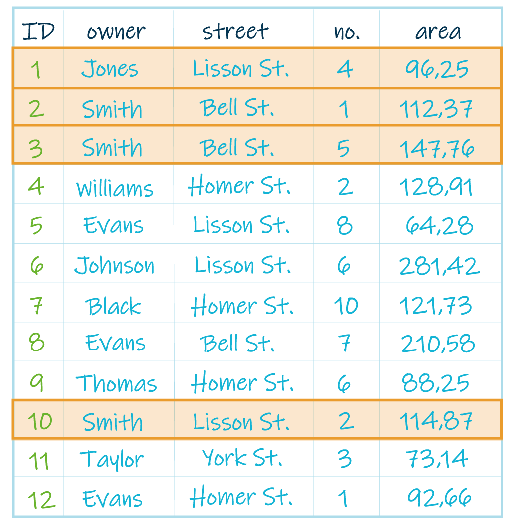
"owner" = 'Smith' OR "owner" = 'Jones'
Complex query - operator AND
AND - result of query contains features which have two attributes at the same time
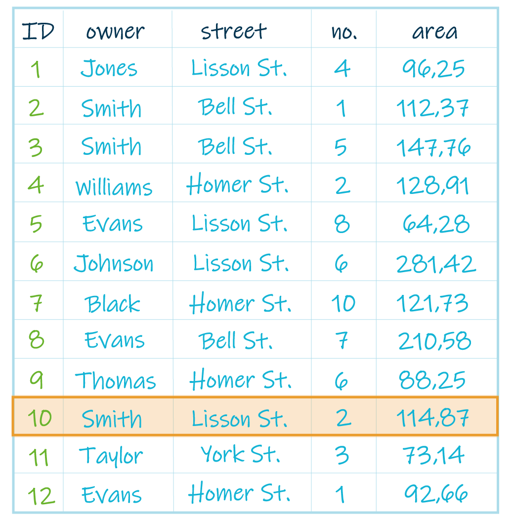
"owner" = 'Smith' AND "street" = 'Lisson St.'
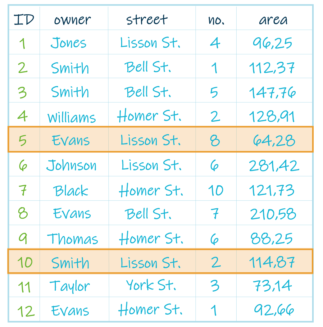
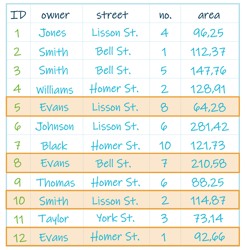
Complex queries
 |
 |
|
("owner" = 'Evans' OR "owner" = 'Smith') AND "street" = 'Lisson St.' |
"owner" = 'Evans' OR ("owner" = 'Smith' AND "street" = 'Lisson St.') |
4.2 | Spatial query
Spatial query - definition
Query is a request to select features or records from a database. Often written as a statement or logical expression.
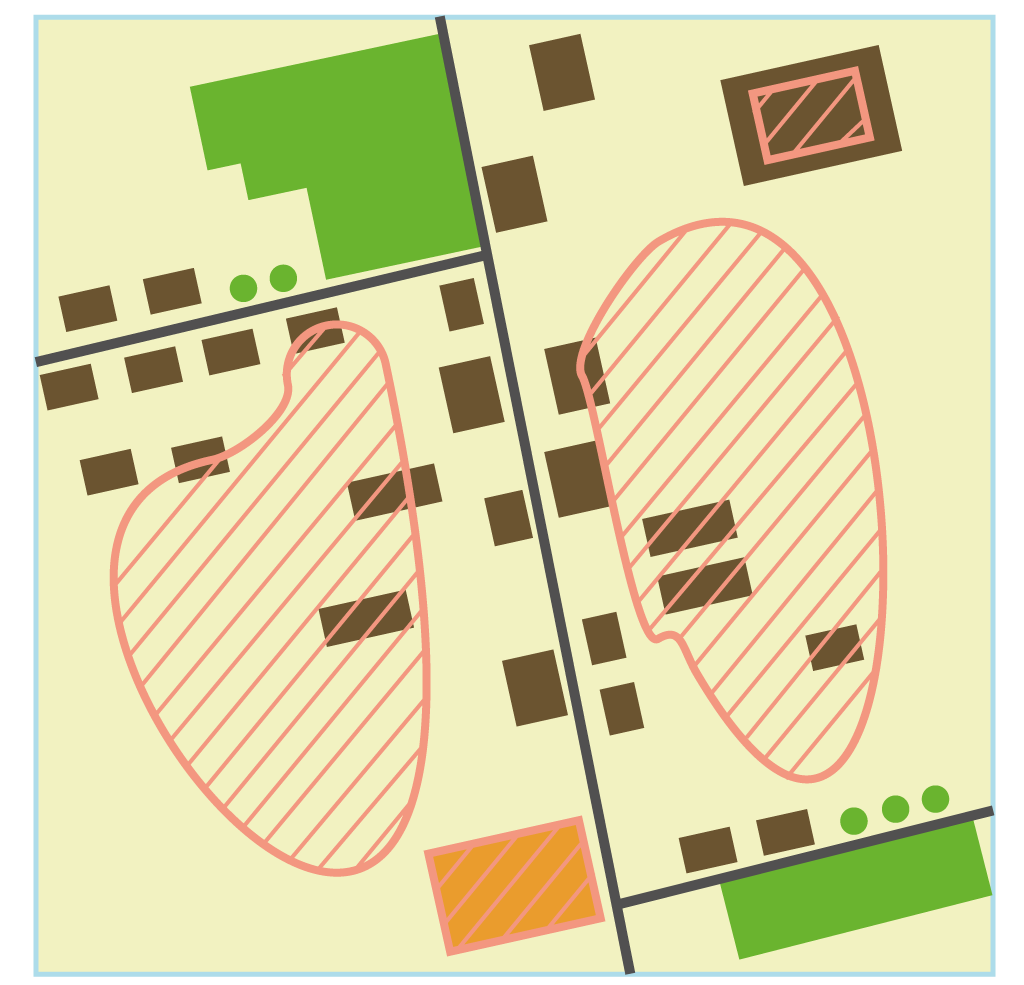
Spatial query is the process of searching and retrieving records of features in a database based on location or spatial relationship.
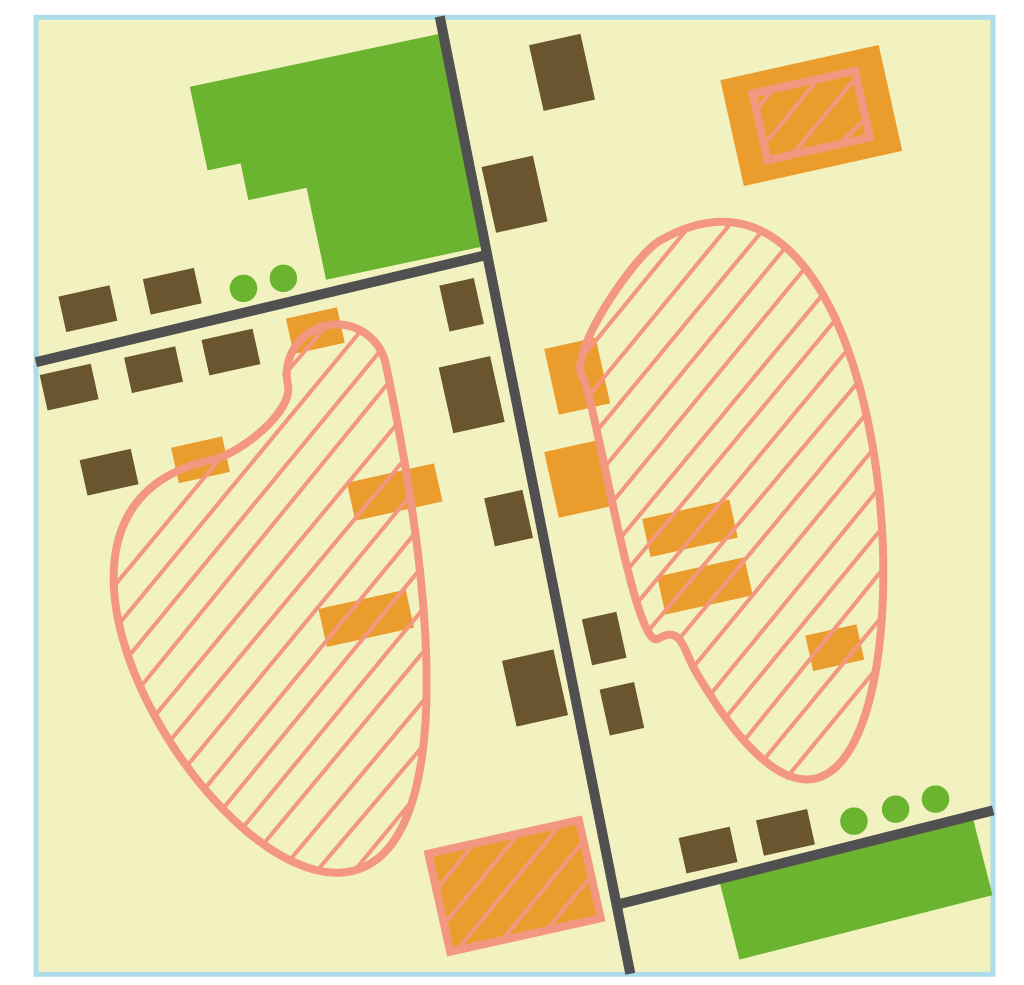
Basic spatial relations
Spatial relationships between objects: Theoretical example: different spatial relations between objects A (buildings) and objects B (landslides) |
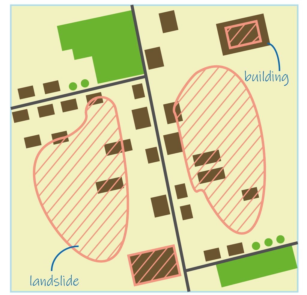 |
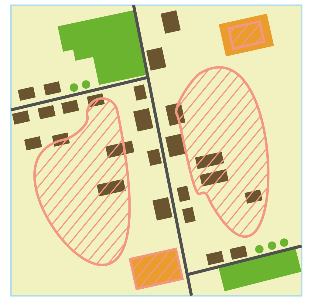
Operator: disjoint
Select: buildings located outside of the landslide Spatial relation: objects A and B do not have any common space Result of request: 17 buildings |
 |
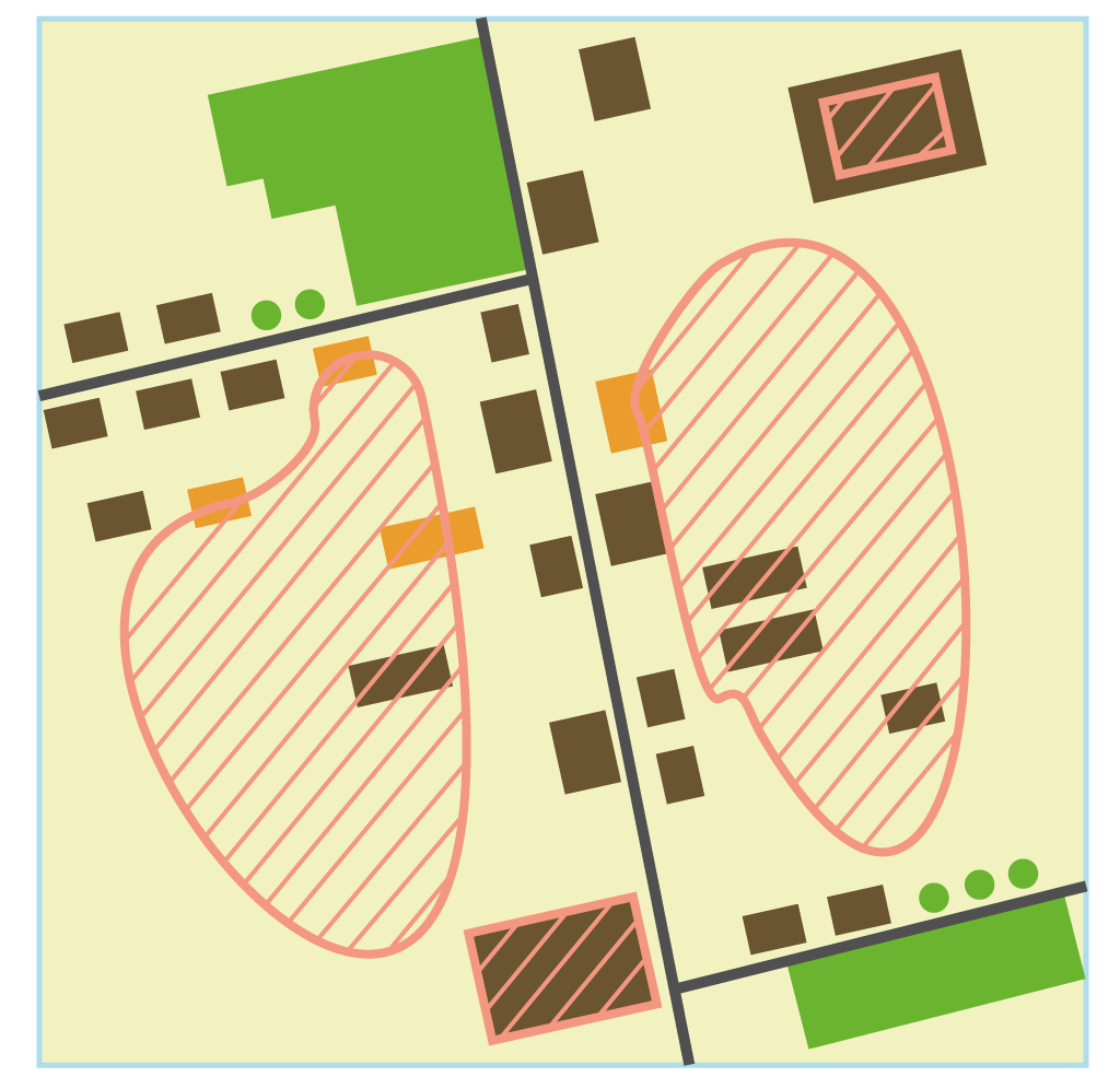
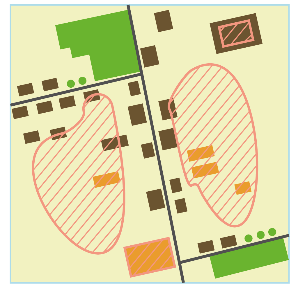
Operator: overlaps
Select: buildings located partially within the landslide Spatial relation: objects A and B overlap partially, but are not completely contained by each other Result of request: 4 buildings |
 |
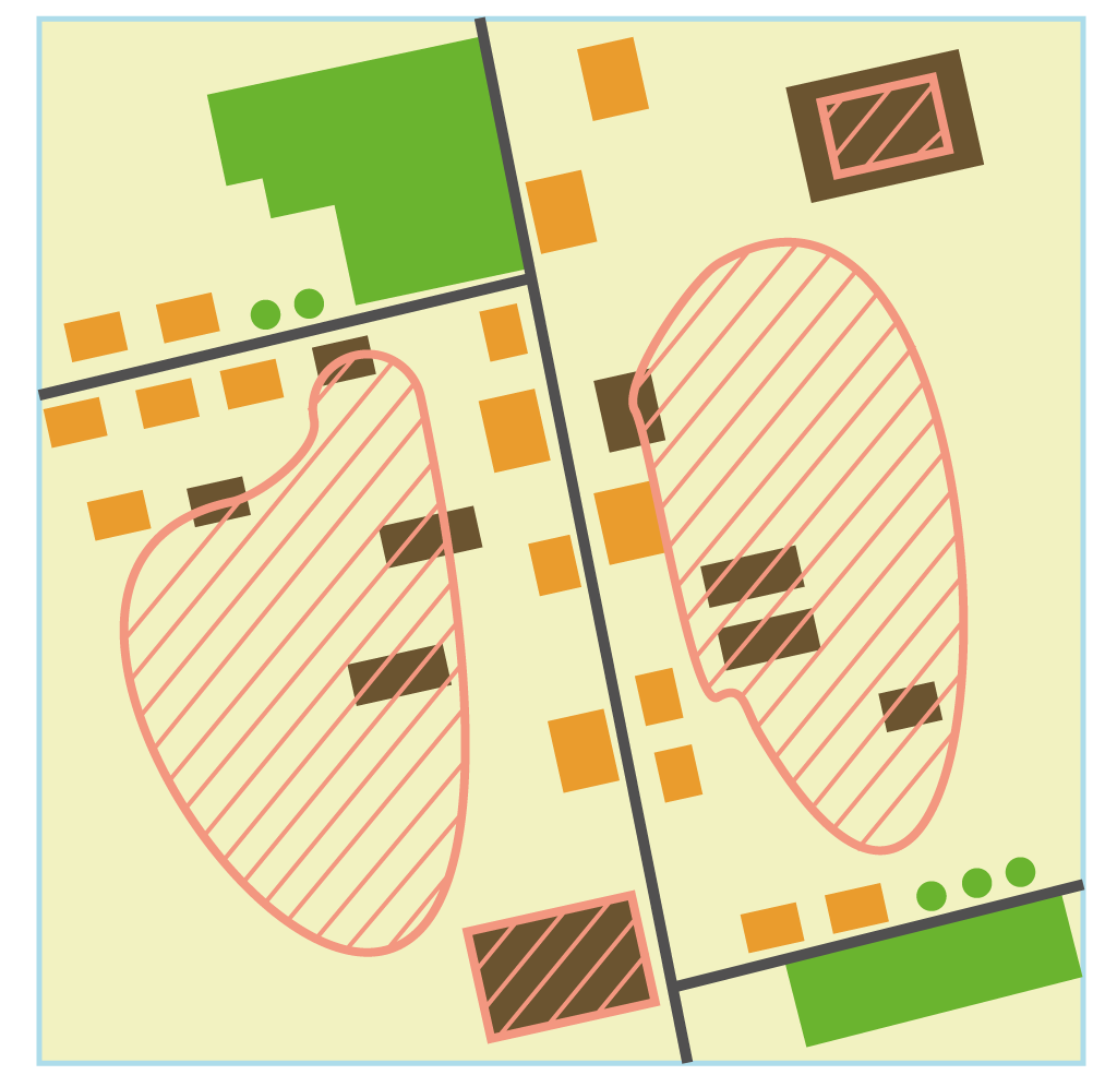
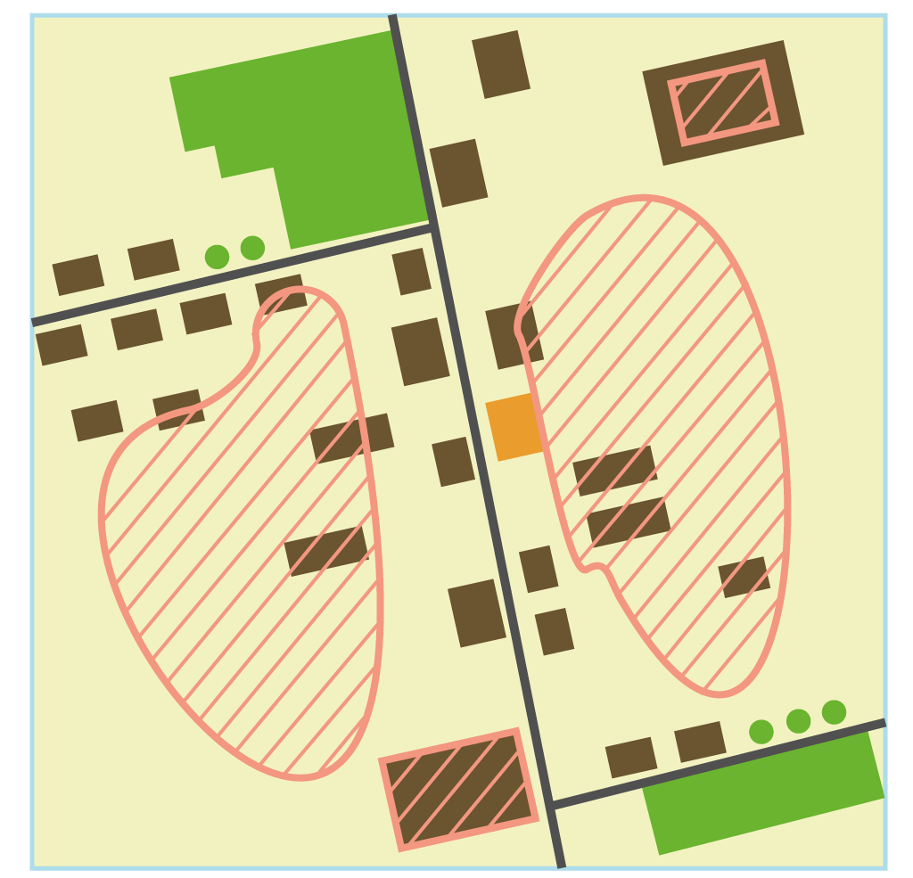
Operator: intersects
Select: buildings located either fully or partially within the landslide Spatial relation: objects A and B share any portion of space Result of request: 11 buildings |
 |
Operator: contains
Select: buildings containing the landslide (theoretical case) Spatial relation: objects A contain objects B within their boundaries Result of request: 2 buildings |
 |
Operator: within
Select: buildings located fully within the landslide Spatial relation: objects A are completely inside objects B Result of request: 5 buildings |
 |
Operator: touches
Select: buildings touching the border of the landslide Spatial relation: objects A and B have at least one point in common, but their interiors do not intersect Result of request: 1 building |
 |
Operator: equals
Select: buildings with the same geometry as the landslide (theoretical case) Spatial relation: objects A and B have strictly equal geometries Result of request: 1 building |
 |
4.3 | Geoprocessing
Buffer
A buffer is a zone around a map feature measured in units of distance or time.
A buffer is useful for proximity analysis.
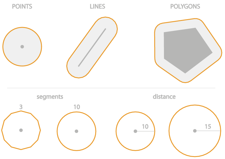
Buffer tool and its parameters
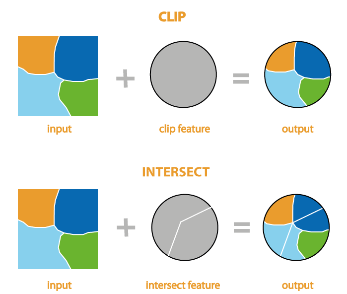
Clip and Intersect
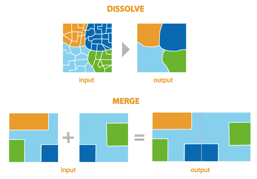
Dissolve and Merge
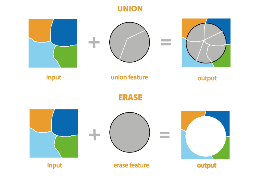
Union and Erase
5 | Data visualization
Introduction to GIS
| # | Content |
| 5.1 | Data visualization |
| 5.2 | Creating maps |
5.1 | Data visualization
Data visualization
Data visualization is the graphic representation of data.
Spatial data is usually presented in the form of maps. There are many different types of maps to show different types of information.
In a GIS, one of the most common types of maps are thematic maps that can represent a variety of information including climate, vegetation, population, and many others.
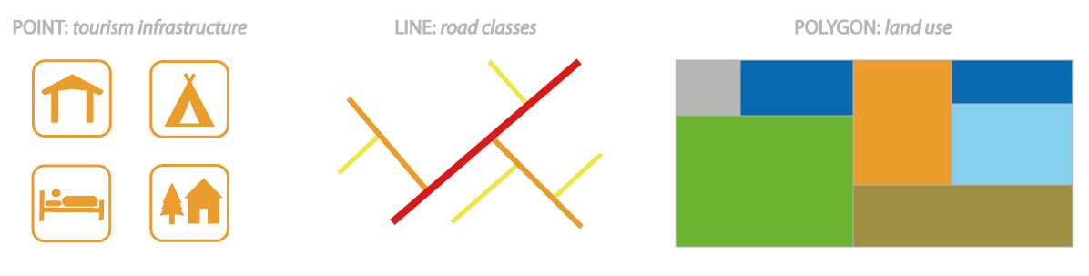
Main ways to represent spatial data
A single vector layer can be represented in different ways.
A GIS software provides many different methods of symbolization, e.g.:
- single symbol
- unique values
- graduated colors
- graduated symbols
- charts
- dot density
- heat map
You can also set other layer display properties such as:
- transparency (0-100%),
- labels: names of objects (e.g. names of rivers, streets) and numbers,
- display scale.
Single symbol
Single symbol applies the same symbol to all features in a layer. This method of symbology is used for representing a layer with only one category.
Properties of symbol according geometry types: |
 |
Unique values
Unique values symbolize qualitative categories of values. Unique value symbology can be based on one or more attribute fields in the dataset, or you can write an expression to generate values on which to symbolize.
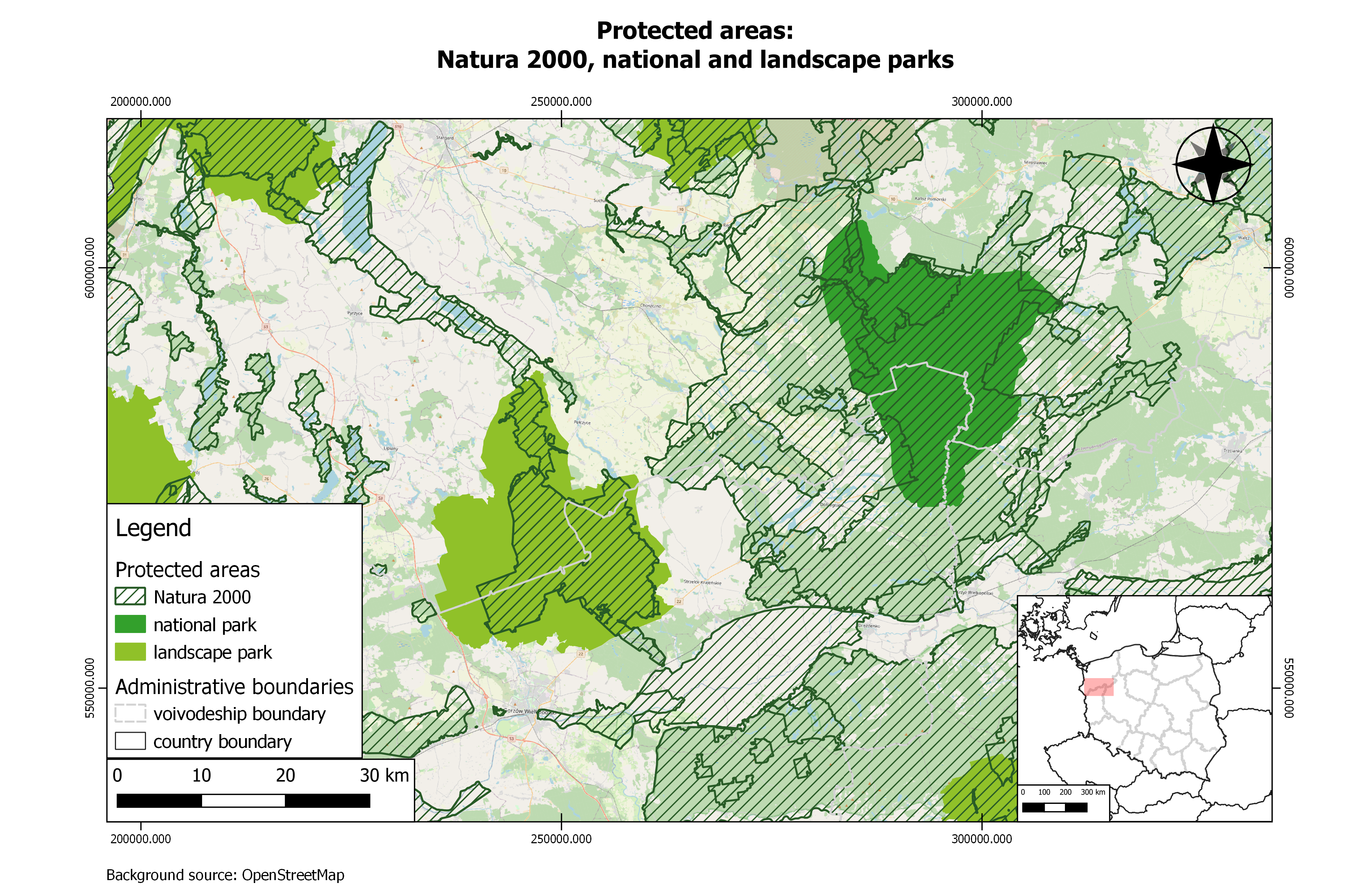
Graduated colors
Graduated colors symbology is used to show a quantitative differences in features by varying the color of symbols. Data is classified into ranges that are each assigned a different color to represent the range.
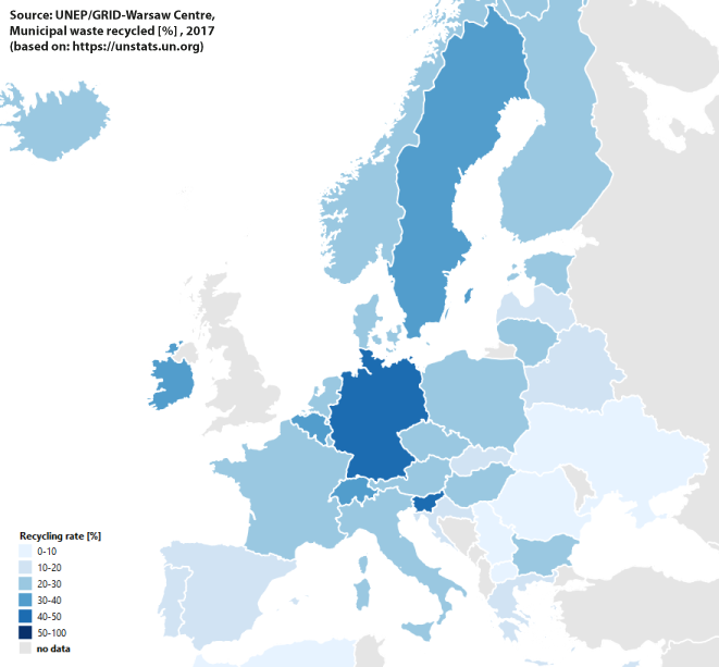
An example of graduated color map
Graduated symbols
Graduated symbols symbology is used to show a quantitative differences in features by varying the size of symbols. Data is classified into ranges that are each assigned a symbol size to represent the range.
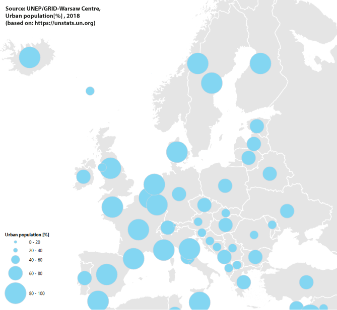
An example of graduated symbol map
Chart
A chart is a type of statistical graphic that represents data.
Chart symbology show quantitative differences between attributes, with each part of the chart representing an attribute value that contributes to the overall whole set of values.
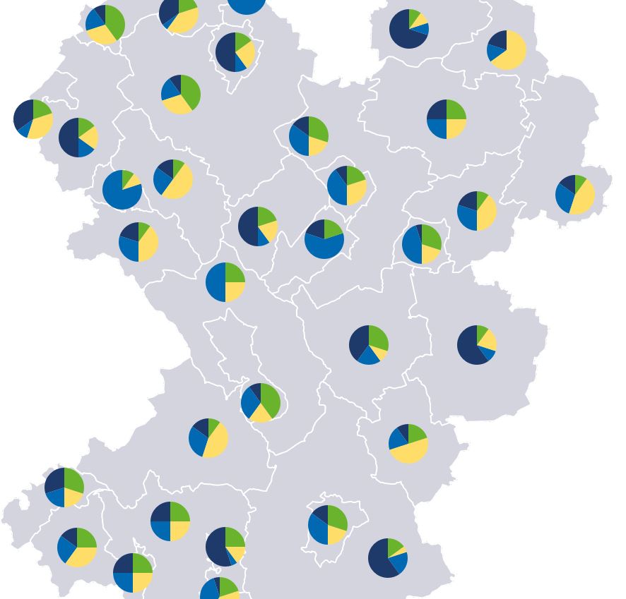
An example of chart map
5.2 | Creating maps
Map-making step by step
- Content (select layers: turn on/turn off the relevant layers, add missing thematic layers, rename layers)
- Symbology (choose the method of data visualization, add labels)
- View setting (determine the scale of map content display, adjust the extent of the map window)
- Map composition (create a new project in the print layout, compose a thematic map by adding elements such as map frame, legend, scale etc.)
- Print (set printout parameters, save print project)
Map elements
A map can be composed of many different map elements.
They may include:
- main map body
- inset or location map(s)
- legend - a visual explanation of the symbols used on the map
- title - a subject of the map
- map scale - the ratio of a distance on the map to the corresponding distance on the ground
- orientation indicator - the relationship between the directions on the map and the corresponding compass directions in reality (e.g. north arrow, graticule)
- map source and additional information (text, graphic, data source, credits, authors, etc.)
Map
Basic principles of map creation (1/2)
- Balance involves the organization of the map and other elements on the page. The various parts of a map layout should be distributed in a way that their weight is centered around the visual center of the map. Four types of balance: symmetrical, asymmetrical, radial and mosaic.
- Legibility is the ability to be seen and understood. Legibility depends on good decision-making for selecting symbols and choosing sizes so that the results are easily seen and understood.
- Clarity is the ease of recognition of map elements.
Basic principles of map creation (2/2)
- Visual contrast relates how map features and page elements contrast with each other and their background.
- Figure-ground organization on the map is distinction between one or more objects of interest in the foreground (figure) and the remainder of the map (the ground). Using figure-ground contrast is an effective method to focus the map reader's attention on the most important elements of the map.
- Hierarchal organization is to "separate meaningful characteristics and to portray likenesses, differences, and interrelationships"
(Robinson, et al,. 1995) . The internal graphic structuring of the map (and the page layout) is fundamental to helping people read your map.
Thank you for your attention!