Introductory Course
Fundaments of Optical Remote Sensing
Module 1
Matter Radiation Interaction
Remote sensing or what ?
In our case we will consider only Space Technologies suitable for:
Telerilevamento
(from the Vocabulary of Italian Language, Treccani, 2000)
Télédétection
in French language
"...long-distance detection of the appearance and the situation of a territory, particularly its
weather and environmental conditions ... its natural resources (forests, water, etc..) usually by air or, now, almost
exclusively from artificial satellites... "equipped with sensors sensitive to different types of electromagnetic waves.

|
|
|
| SONAR (Sound Navigation And Ranging) | LIDAR (LIght Detection And Ranging) | RADAR (RAdio Detection And Ranging) |

THEORETICAL TOOLS:
Basic Definitions and Physical Laws
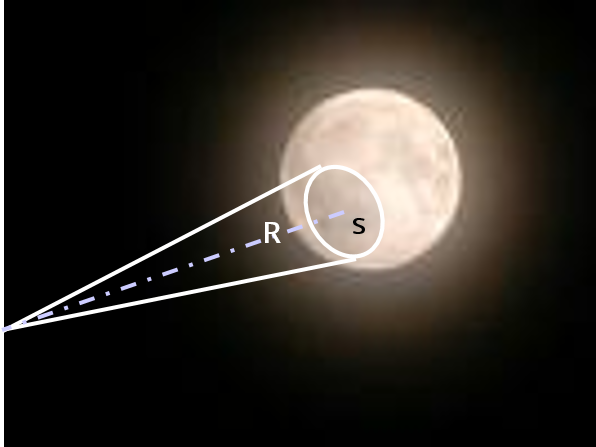
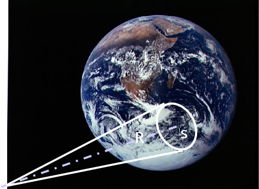
Solid angle Ω
The solid angle \(\Omega\) is the ratio of the area \(\sigma\) intercepted on the surface of a sphere of radius R by a cone with the vertex in the center of the sphere and the square of the sphere radius (\(R^2\)). The measuring unit is the steradian [sr]
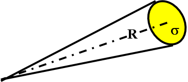 \(\bbox[5px, border: 2px solid #2D5595]{\Omega = \frac{\sigma}{R^2}}\)
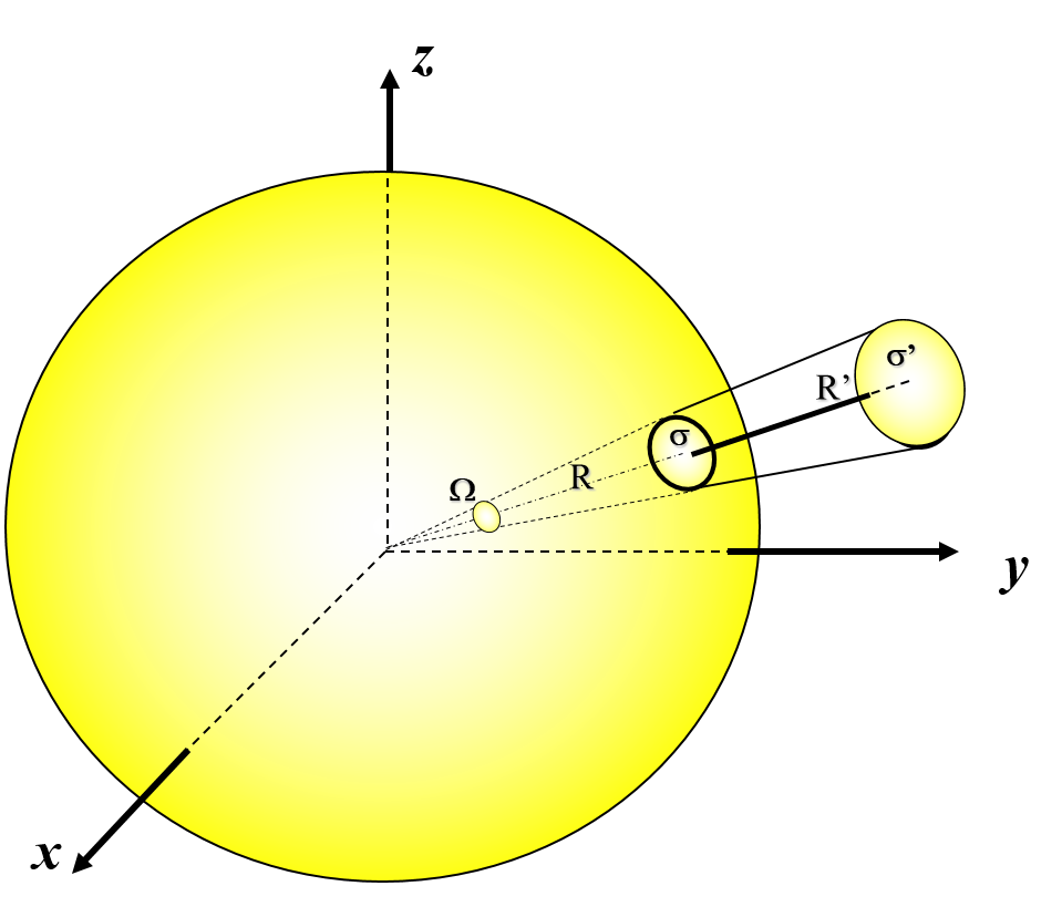
\(\Omega=\frac{\sigma}{R^2}=\frac{\sigma '}{R^{ '2}}\)
\(\Omega = \frac{\sigma}{R^2}=\frac{4\pi R^2}{R^2}=4\pi sr\)
Monochromatic Radiance
The monochromatic radiance represents the energy collected in a unit of time and solid angle when the unit of surface of a detector is crossed by e.m. radiation of wavelength in between \(\lambda\) and \(\lambda + d\lambda\) and directed orthogonally to the surface A.
Hortogonally Incident Radiation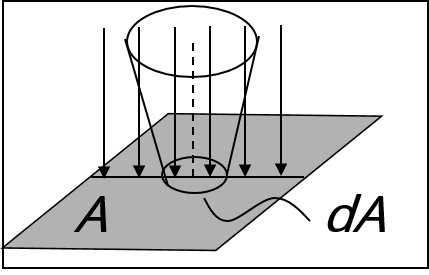
\(\bbox[5px, border: 2px solid #2D5595]{I_\lambda = \frac{dE_\lambda}{dt \cdot dA \cdot d\lambda \cdot d\Omega}} \) \( [I_\lambda]=[Watt \cdot m^{-2} \mu m^{-1} sr^{-1}]\)
\( dE_\lambda=\)energy, [J]; \(dt=\)time[s]; \(dA=\)collecting area [\(m^2\)];
\(d_\lambda=\)wavelength interval [\(\mu m\)]; \(d\Omega=\)collecting solid angle [ster]
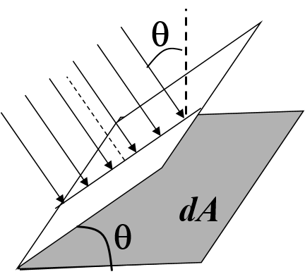
In general \( \Theta \ne 0\)
\(\bbox[15px, border: 2px solid #003366]{I_\lambda = \frac{dE_\lambda}{dt \cdot dA \cdot \cos{\Theta} \cdot d\lambda \cdot d\Omega}} \)

From sensors to radiation sources
To the sensor
|
From the source

|
EXEMPLE:THE SUN |
|
RADIANT POWER
\(f = dE / dt\) [W] |
LUMINOSITY
\(f = dE / dt\) [W] |
Ex.: Sun Luminosity
\(f = 3.90 \times 10^{26} W\) |
|
IRRADIANCE
\(F = dE / dt / dA\) \([W m^{-2}]\) |
(RADIANT) EXISTANCE
\(F = dE / dt /dA\) \([W m^{-2}]\) |
Ex: Sun Exitance for a Sun radius \(R = 7 \times 10^8m\)
\(F(Sun) = \frac{3.90 \times 10^{26}}{4\pi (7 \times 10^8)^2} = 6.34 \times 10^7 W m^{-2}\) |
|
RADIANCE
\(I = dE / dt / d\Omega\) \([W m^{-2}st^{-1}]\) |
RADIANCE (BRILLANCE)
\(I = dE / dt / dA / d\Omega\) \([W m^{-2}st^{-1}]\) |
Ex.: Radiance leaving from Sun surface (assumed Lambertian i.e. isotropic) \(I = F/\pi = 2.02 \times 10^7 W m^{-2} st^{-1}\) |
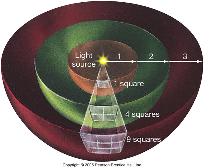
Inverse square law
\(f_\lambda=\frac{dE_\lambda}{dt \cdot d\lambda \cdot}=\int F_\lambda dA = \int dA \int I_\lambda(\Theta, \phi) cos\Theta d\Omega\)
\(f_\lambda =\) cost \(\leftarrow\) cons. of the Energy
\(f_\lambda = F_\lambda \int dA = F_\lambda \cdot 4\pi d^2 = F_\lambda^{'} \cdot 4\pi d^{'2} = f_\lambda^{'}\)
for a punctual Lambertian source
\(F_\lambda (d) = \frac{f_\lambda}{4\pi d^2}\)
\(F_\lambda(d) \propto \frac{f_\lambda}{d^2}\)
\(\frac{F_\lambda (d_2)}{F_\lambda (d_1)} = \frac{d_1^2}{d_2^2}\)
Blackbody Radiation
 Planck's function
\(\bbox[5px, border: 2px solid #003366]{B_\lambda(T) = \frac{2~~h~~c^2}{\lambda^5(e^{\frac{h~~c}{\lambda~~k~~T}}-1)}}\)
\(B_\lambda(T)=\) monochromatic radiance emitted at the
wavelength \(\lambda\) by a blackbody at the absolute
temperature \(T [W/m^3]\)
\(c=2.998 \cdot 10^8 m/s\) speed of light in the vacuum
\(h=6.626 \cdot 10^{-34} Js\) Planck’s constant
\(k=1.380 \cdot 10^{-23} J/K\) Boltzman constant
Reyleigh-Jeans approximation
\(B_\lambda=\frac{2~~h~~c^2}{\lambda^5{(e^{\frac{h~~c}{\lambda~~k~~T}}-1)}}\) if \(\lambda>0.001m\) \(T\)~\(300K\)
Planck
\(x=\frac{h~~c}{\lambda~~k~~T}\rightarrow 0\)
\(e^x = 1 + x + ....\) Taylor
\(e^{\frac{h~~c}{\lambda~~k~~T}}\approx 1 + \frac{h~~c}{\lambda~~k~~T}\)
\(B_\lambda(T)\approx \frac{2~~h~~c^2}{\lambda^5(1+\frac{h~~c}{\lambda~~k~~T}-1)}\)
\(\bbox[5px, border: 1px solid #003366, #CCCCFF]{B_\lambda(T) \approx \frac{2 k c T}{\lambda^4} \propto T}\)
Reyleigh-Jeans
Emissivity
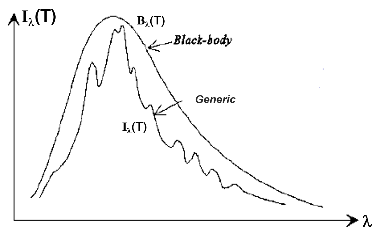 \(B_\lambda(T) = \frac{2~~h~~c^2}{\lambda^5(e^{\frac{h~~c}{\lambda~~k~~T}}-1)}\)
Brightness Temperature
Planck's function
\(\bbox[5px, border: 2px solid #003366]{B_\lambda(T) = \frac{2~~h~~c^2}{\lambda^5(e^{\frac{h~~c}{\lambda~~k~~T}}-1)}}\)
Blackbody Temperature
\(\bbox[5px, border: 2px solid #003366]{T = \frac{hc}{\lambda k} \frac{1}{\ln[1+\frac{2~hc^2}{\lambda^5 B_\lambda(T)}]}}\)
Brightness Temperature
\(\bbox[5px, border: 2px solid #003366]{T_B = \frac{hc}{\lambda k} \frac{1}{\ln[1~+~\frac{2~hc^2}{\lambda^5 I_\lambda(T)}]}}\)

Brightness Temperature
Exercise: Moon surface temperature
\( T_s = \frac{hc}{\lambda~k} \frac{1}{\ln[1~+~\frac{2~hc^2}{\lambda^5~I_\lambda(T)}]} \)
\( \bbox[5px, border: 2px solid #003366]{I_{\lambda=10\mu} = 3 \cdot 10^4 erg \cdot s^{-1} \cdot cm^{-2} \mu m^{-1} sr^{-1}}\)
monochromatic radiance emitted at the
wavelength \( \lambda = 10\mu \) by he Moon surface
\( c\sim 3 \cdot 10^{10} cm/s\) speed of light in the vacuum
\( h\sim 6,6 \cdot 10^{-27} erg \cdot s\) Planck's constant
\( k\sim 1,4 \cdot 10^{-16} erg/K\) Boltzman constant
Brightness Temperature
\(=\frac{6,6~\cdot~3~\cdot~10^2}{1,4}\frac{1}{\ln[1~+~\frac{2~\cdot~6,6~\cdot~9}{3}sr]}K= \frac{6,6~\cdot~3~\cdot~10^2}{1,4}\frac{1}{3,7}K \approx 382~K\)
Brightness Temperature
Exercise: Earth's surface temperature
\( \bbox[5px, border: 2px solid #003366]{I_{\lambda=10\mu} = 10^4 erg \cdot s^{-1} \cdot cm^{-2} \mu m^{-1} sr^{-1}}\)
monochromatic radiance emitted at the
wavelength \( \lambda = 10\mu \) by he Moon surface
\( c\sim 3 \cdot 10^{10} cm/s\) speed of light in the vacuum
\( h\sim 6,6 \cdot 10^{-27} erg \cdot s\) Planck's constant
\( k\sim 1,4 \cdot 10^{-16} erg/K\) Boltzman constant
Brightness Temperature
\(=\frac{6,6~\cdot~3~\cdot~10^2}{1,4}\frac{1}{\ln[1~+~\frac{2~\cdot~6,6~\cdot~9}{1}sr]}K= \frac{6,6~\cdot~3~\cdot~10^2}{1,4}\frac{1}{4,8}K \approx 296~K\)
Brightness Temperature
(Reyleigh-Jeans approximation)
Planck's function
\(\bbox[5px, border: 2px solid #003366]{B_\lambda(T) \approx \frac{2~kcT}{\lambda^4} ~\propto~T}\)
Blackbody Temperature
\(\bbox[5px, border: 2px solid #003366]{T \approx \frac{\lambda^4}{2~kc} B_\lambda(T)}\)
\(\bbox[5px, border: 2px solid #2D5595]{T_B\sim\epsilon_\lambda T}\) \(\bbox[5px, border: 2px solid #2D5595]{T_B\leq T}\)
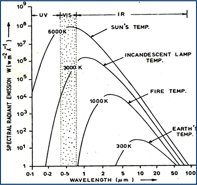
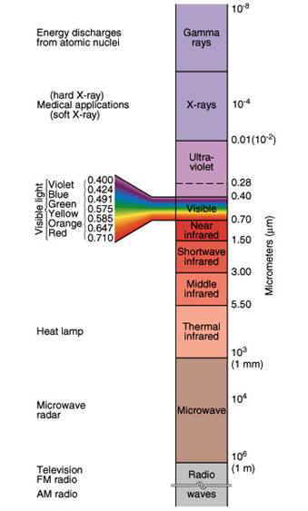
Wien's Displacement Law
\(\bbox[5px, border: 2px solid #2D5595]{\lambda_{MAX}(\mu m)=\frac{2898}{T(K)}}\)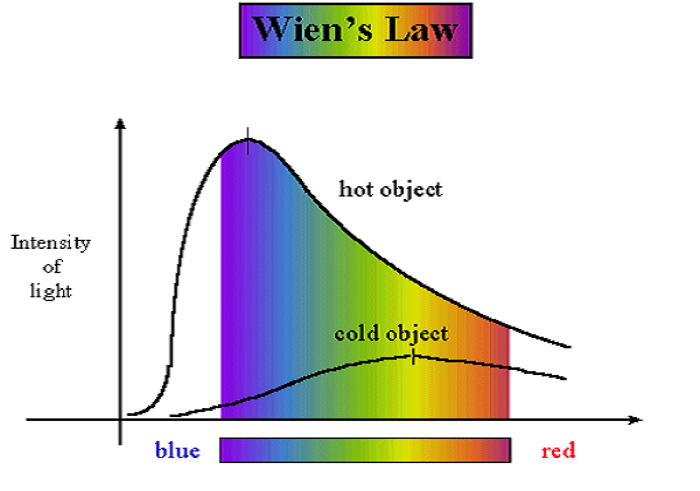

Wien's Displacement Law
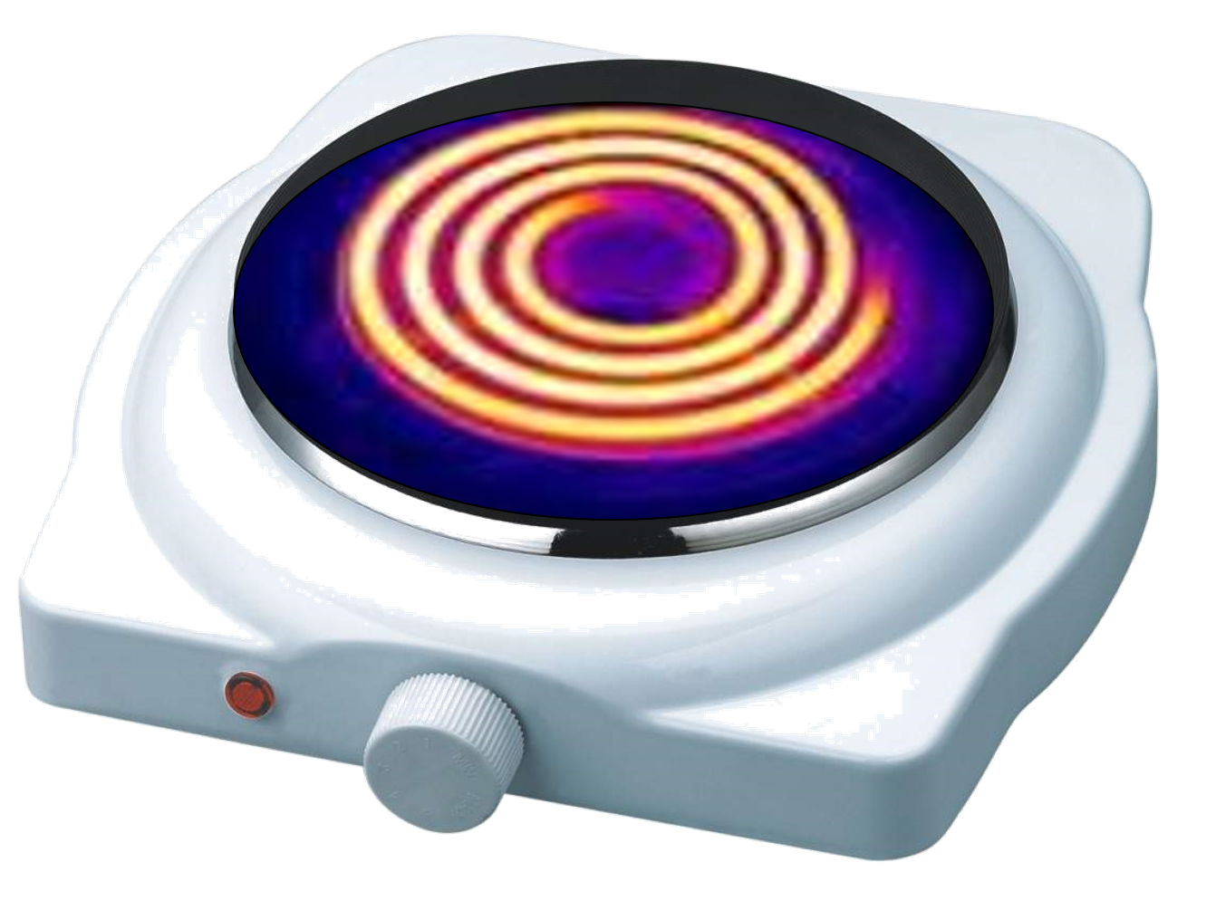
Wien's Displacement Law
Exercise: choosing the best spectral range
Earth surface \(T=300K\)
\(\lambda_{MAX}=10\mu m=\)TIR
fires, lava flows \(T=800~~-1000~K\)
\(\lambda_{MAX}=3-4\mu m = \)MIR
Sun photosphere \(T=6000~K\)
\(\lambda_{MAX} = 0,5\mu m =\) VIS

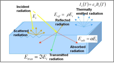
Matter/Radiation Interaction
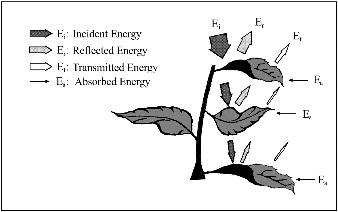
Conservation of the Energy
\(\bbox[5px, border: 1px solid black]{E_i = E_{rif} + E_{ads} + E_{tras}}\)
Matter/Radiation Interaction
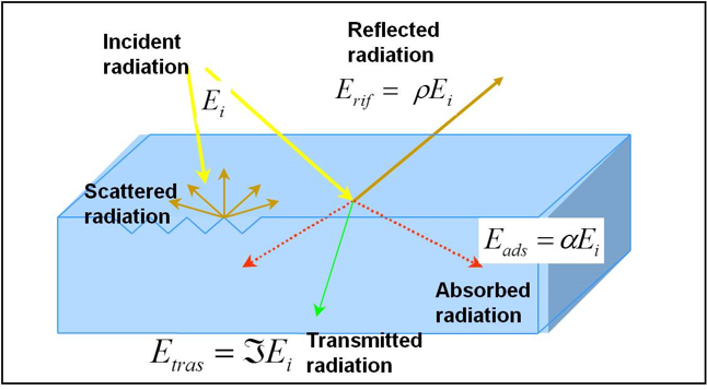
Conservation of the energy
\(\bbox[5px, border: 1px solid black]{E_{rif} + E_{ads} + E_{trans} = E_i}\)
![]()
\(\bbox[5px, border: 1px solid black]{I_\lambda^R + I_\lambda^A + I_\lambda^T = I_\lambda^I}\)
\(\bbox[5px, border: 1px solid black]{\frac{I_\lambda^R}{I_\lambda^I}+\frac{I_\lambda^A}{I_\lambda^I}+\frac{I_\lambda^T}{I_\lambda^I}=\frac{I_\lambda^I}{I_\lambda^I}=1}\)
\(\rho_\lambda=\frac{I_\lambda^R}{I_\lambda^I}\)
\(\alpha_\lambda=\frac{I_\lambda^A}{I_\lambda^I}\)
\(\Im_\lambda=\frac{I_\lambda^T}{I_\lambda^I}\)
Reflectance
Absorbance
Transmittance
 monochromatic
\(\bbox[5px, border: 1px solid black]{\rho_\lambda+\alpha_\lambda+\Im_\lambda = 1}\)
Spectral Signatures in the laboratory
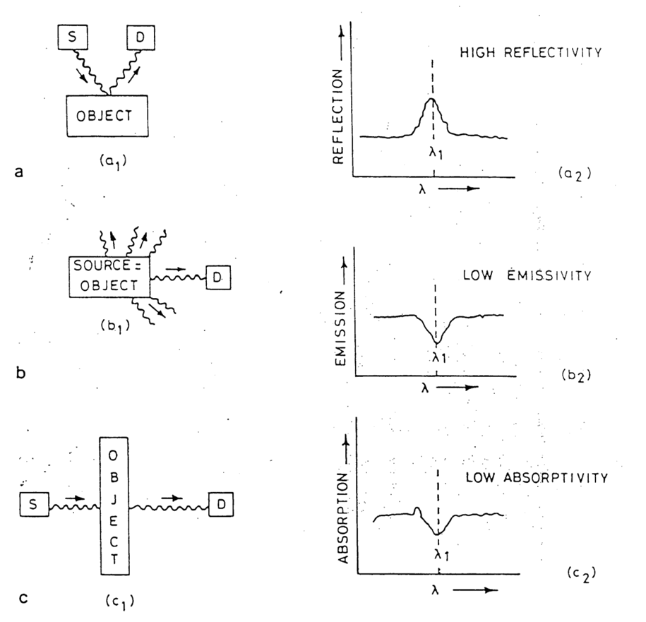
\(\bbox[5px, border: 1px solid black]{\rho_\lambda=\frac{I_\lambda^D}{I_\lambda^S}}\)
\(\bbox[5px, border: 1px solid black]{\epsilon_\lambda=\frac{I_\lambda^D}{B_\lambda(T)}}\)
\(\bbox[5px, border: 1px solid black]{\Im_\lambda=\frac{I_\lambda^D}{I_\lambda^S}}\)
Kirchoff law
at the thermodynamic equilibrium:
\(\bbox[15px, border: 2px solid blue, white]{\epsilon_\lambda = \alpha_\lambda}\) \(\bbox[15px, border: 1px solid black]{\rho_\lambda+\epsilon_\lambda + \Im_\lambda = 1}\)
at the termodynamic equilibrium (Kirchoff)
\(\bbox[15px, border: 1px solid black]{\epsilon_\lambda = \alpha_\lambda = 1 - \rho_\lambda}\)
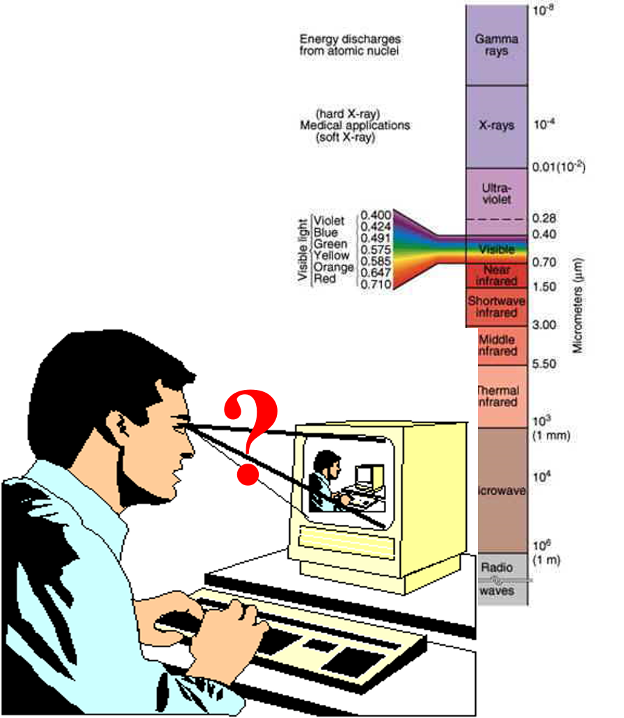
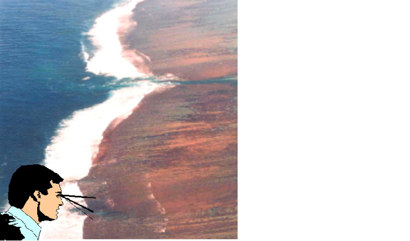
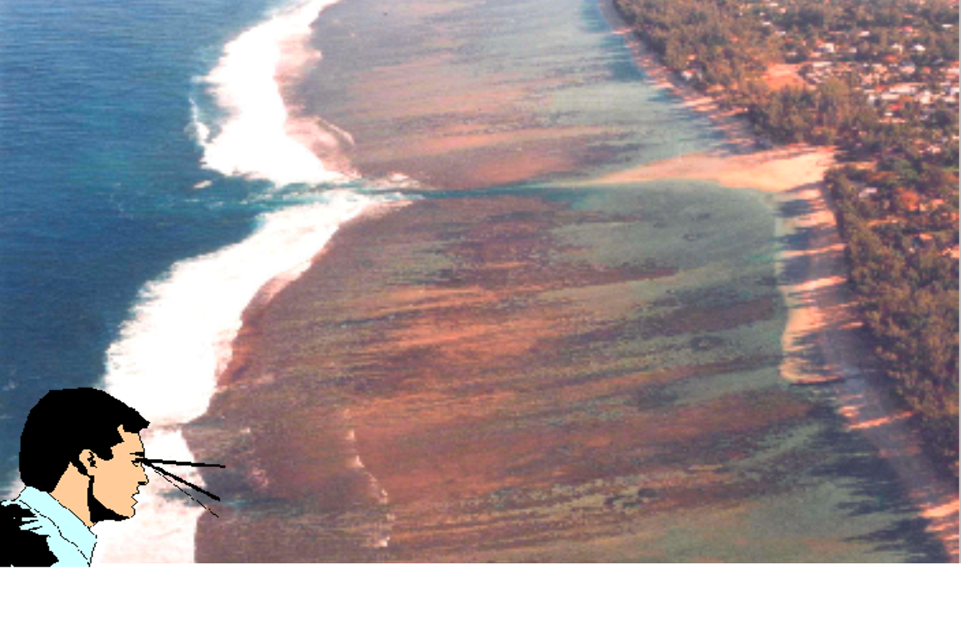
Our daily remote sensing experience
in the visible (VIS) spectral range
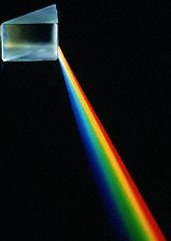
Newton prism and light colors
Our daily remote sensing experience
![]()
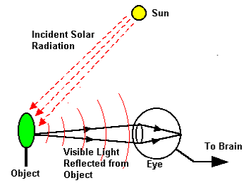
What?
How?
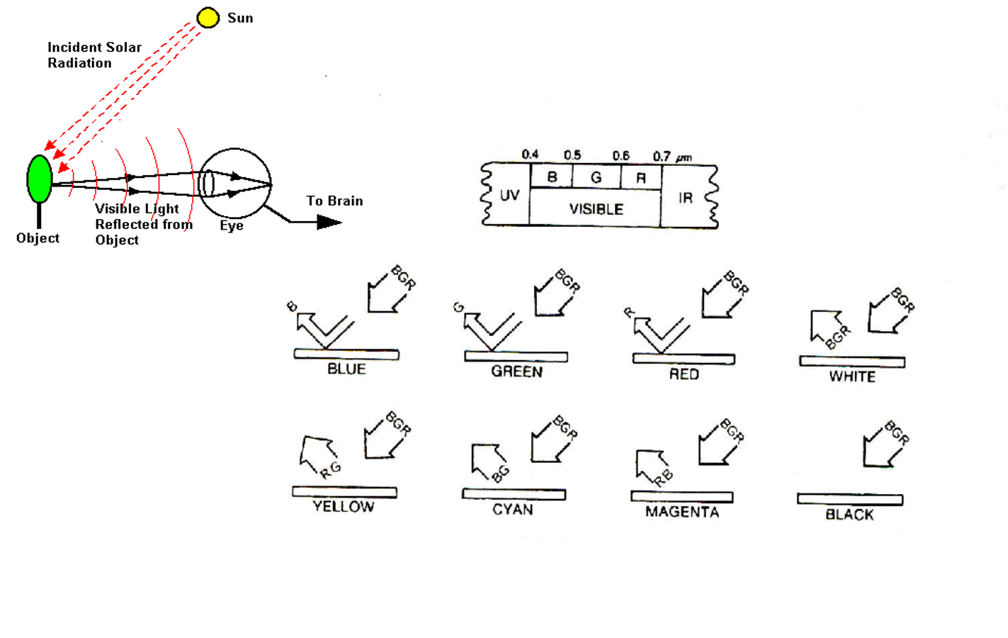
What? better?
How?
Measuring reflectances in the laboratory
\(\bbox[5px, border: 1px solid black]{\rho_\lambda=\frac{I_\lambda^R}{I_\lambda^I}}\)
Reflectance
![]()
Measuring reflectances in the laboratory
![]() \(\bbox[5px, border: 1px solid black]{\rho_\lambda = \frac{I_\lambda^R}{I_\lambda^I}}\)
Reflectance
\(\bbox[5px, border: 1px solid black]{\rho_\lambda = \frac{I_\lambda^R}{I_\lambda^I}}\)
Reflectance
Measuring reflectances in the laboratory
![]()
Beyond visible.
visible and....
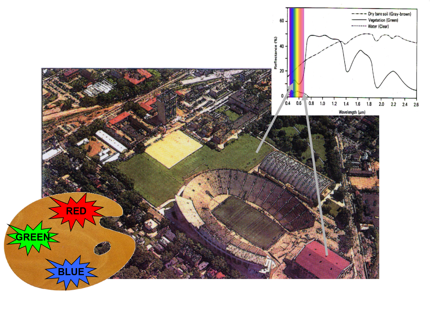
Aerial color picture
beyond visible....
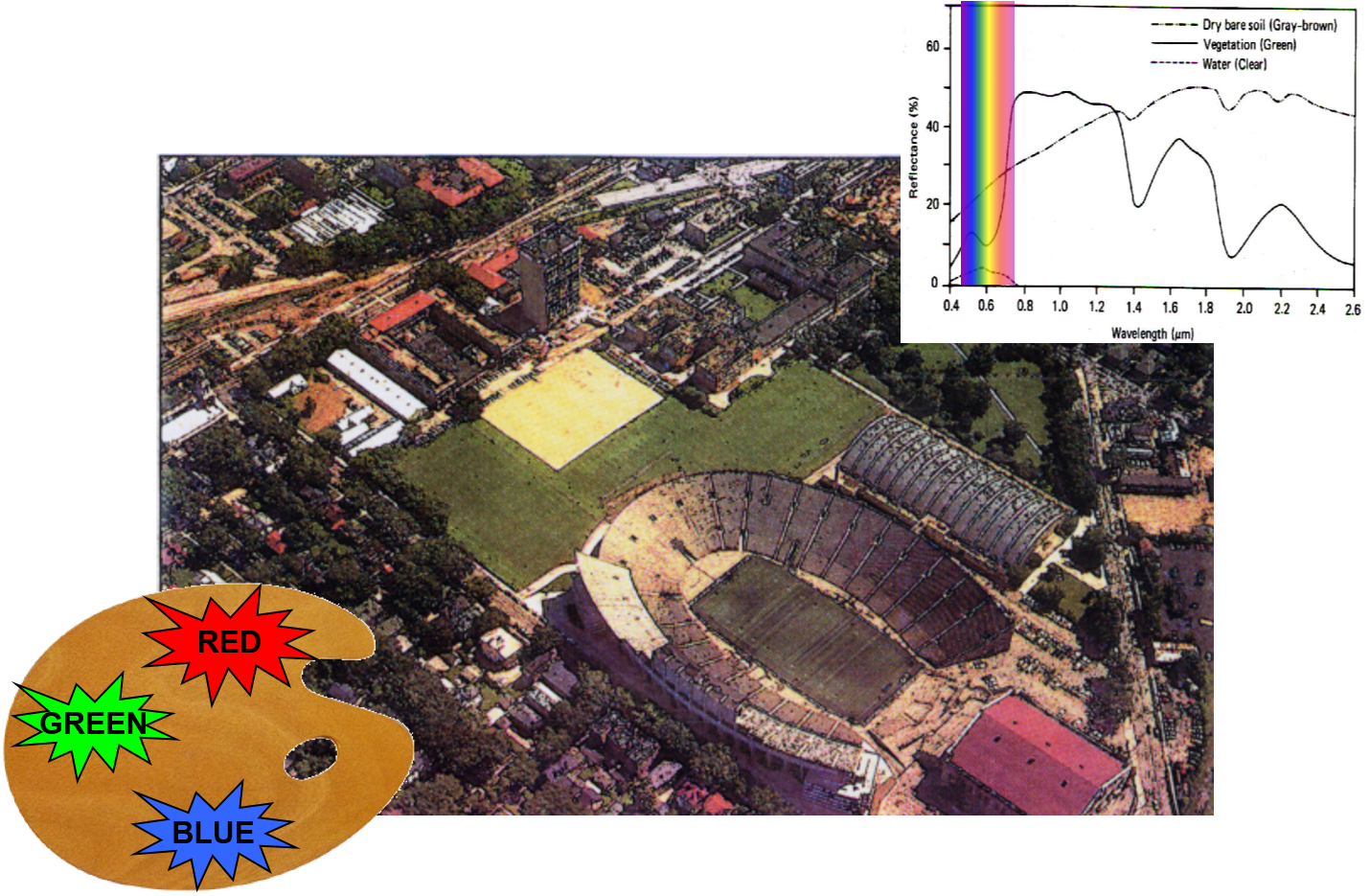
the vegetation “colour” is (near) infrared more than green !
Infrared aerial color picture
TUTORIAL RGB Landsat-ETM
- RGB true color on MODIS image
- RGB false color to enhance vegetation (RED → NIR)
Measuring reflectances in the laboratory
![]()
![]() Which "colors"
Which "colors"
beyond visible?
 Which "colors"
 beyond visible?
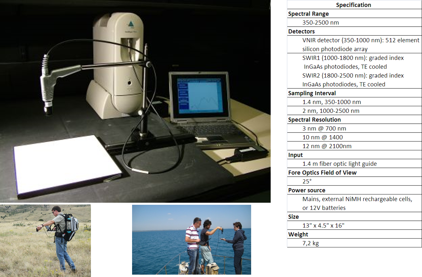
Measuring reflectances in the lab & in the field
(Field Spec ASD Spectrometer)
![]()
(Field Spec ASD Spectrometer)
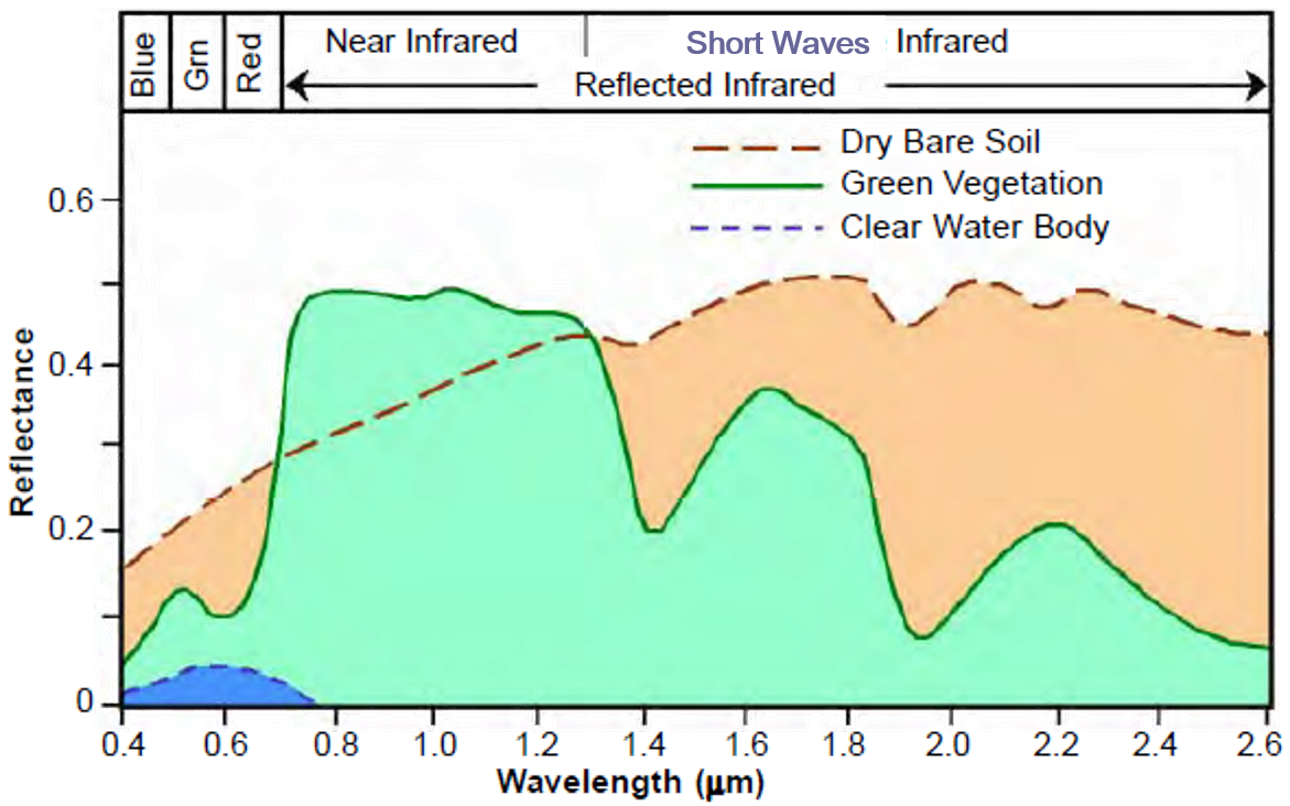
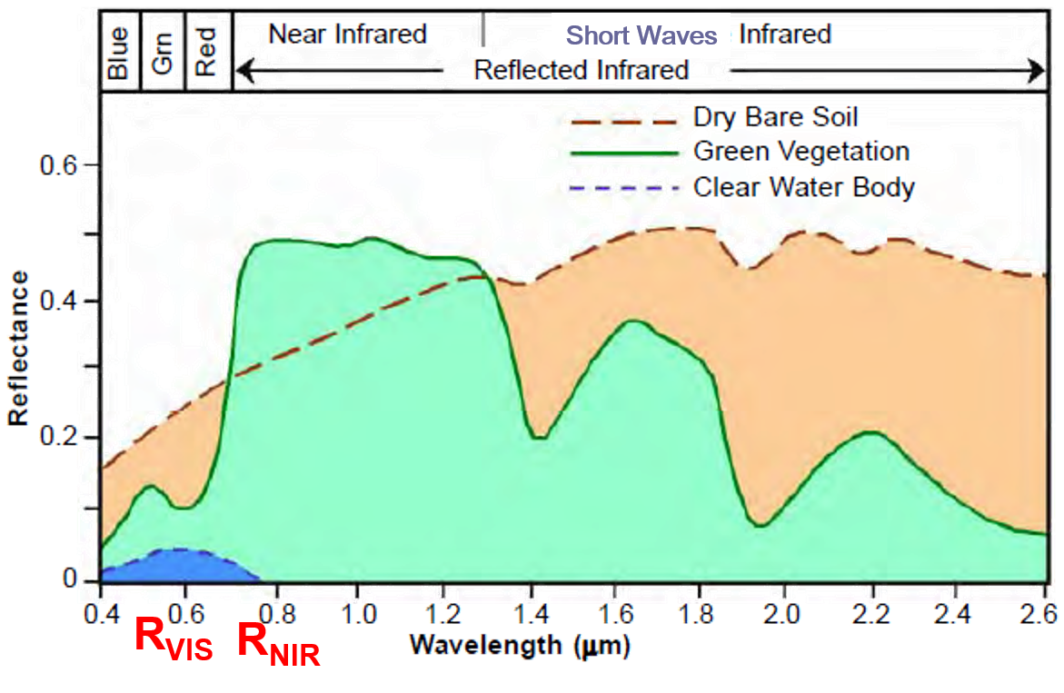
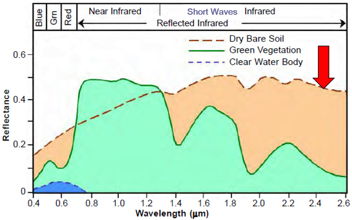
Spectral signatures of soil, water,
vegetation (in reflectance)
![]()
![]()
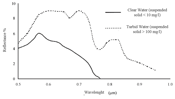
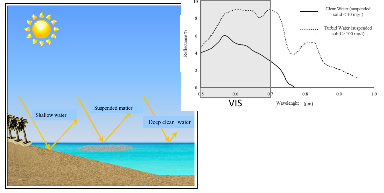
Spectral signature of water
\(\bbox[5px, border: 1px solid black]{\rho_\lambda + \alpha_\lambda + \Im_\lambda = 1}\)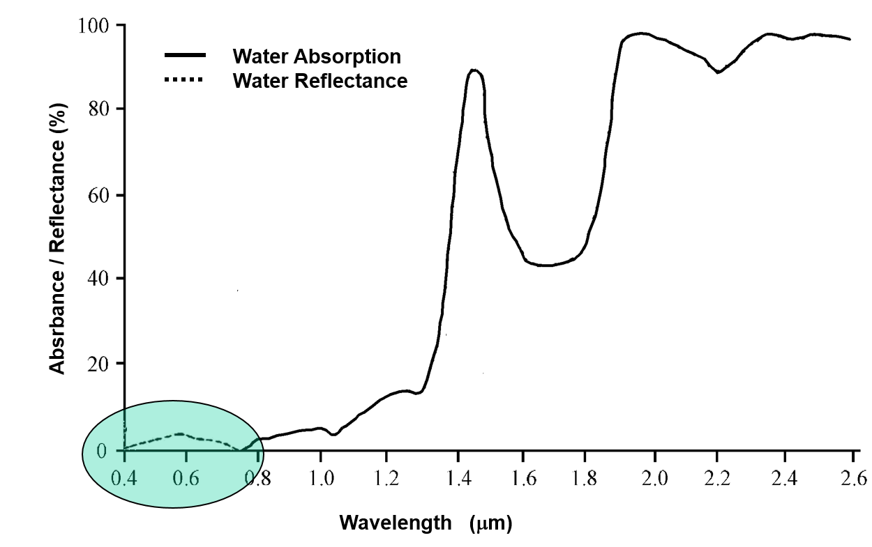
Hight transmittance
Very low transmittance
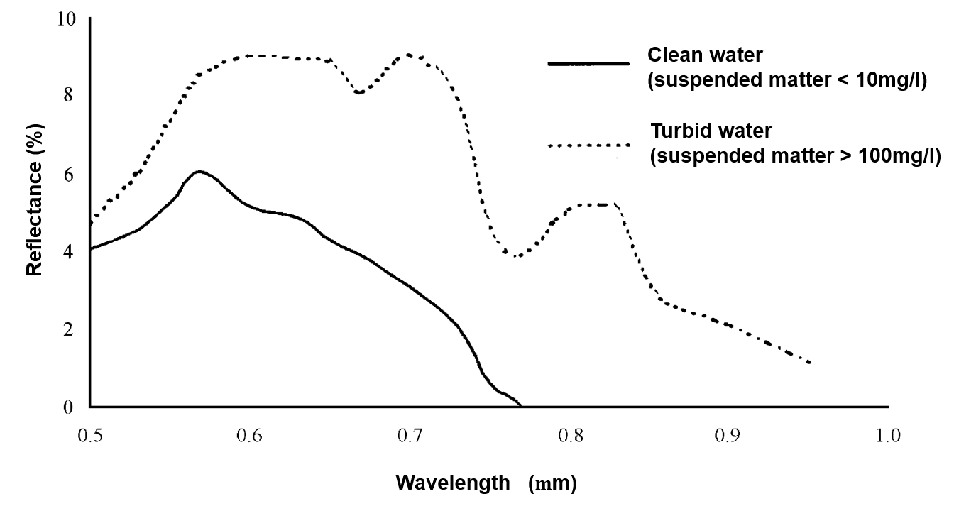
Spectral signatures of (clean/turbid) water
(in reflectance)
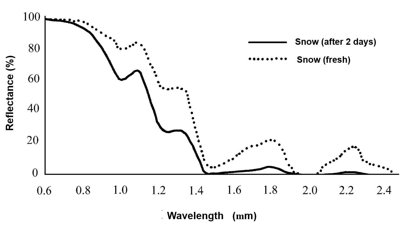
Spectral signatures of snow
(in reflectance)
Spectral signatures of snow and Clouds
(in reflectance)
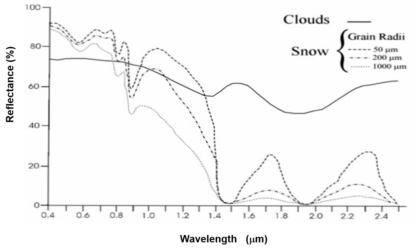
RGB MODIS FOR
DISCRIMINATING SNOW FROM
CLOUDS
Spectral signatures of soil, water,
vegetation (in reflectance)
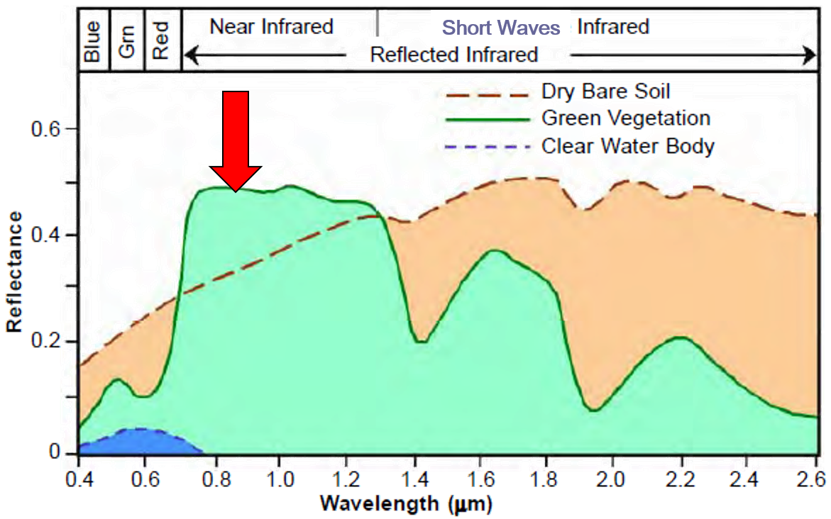
Spectral signatures of vegetation
(in reflectance)
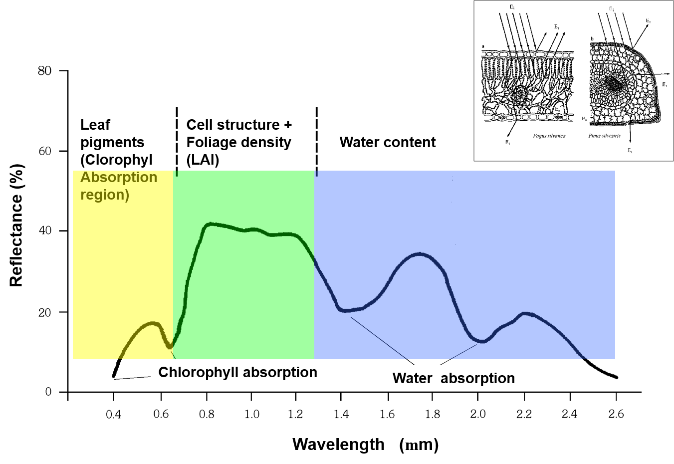
Spectral signatures of vegetation
\(\bbox[5px, border: 1px solid black]{\rho_\lambda + \alpha_\lambda + \Im_\lambda = 1}\)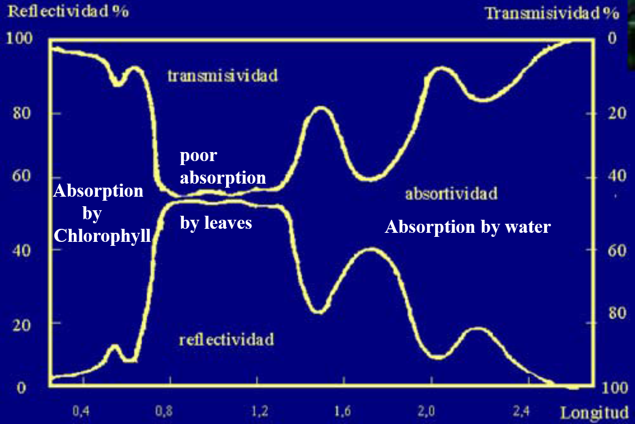
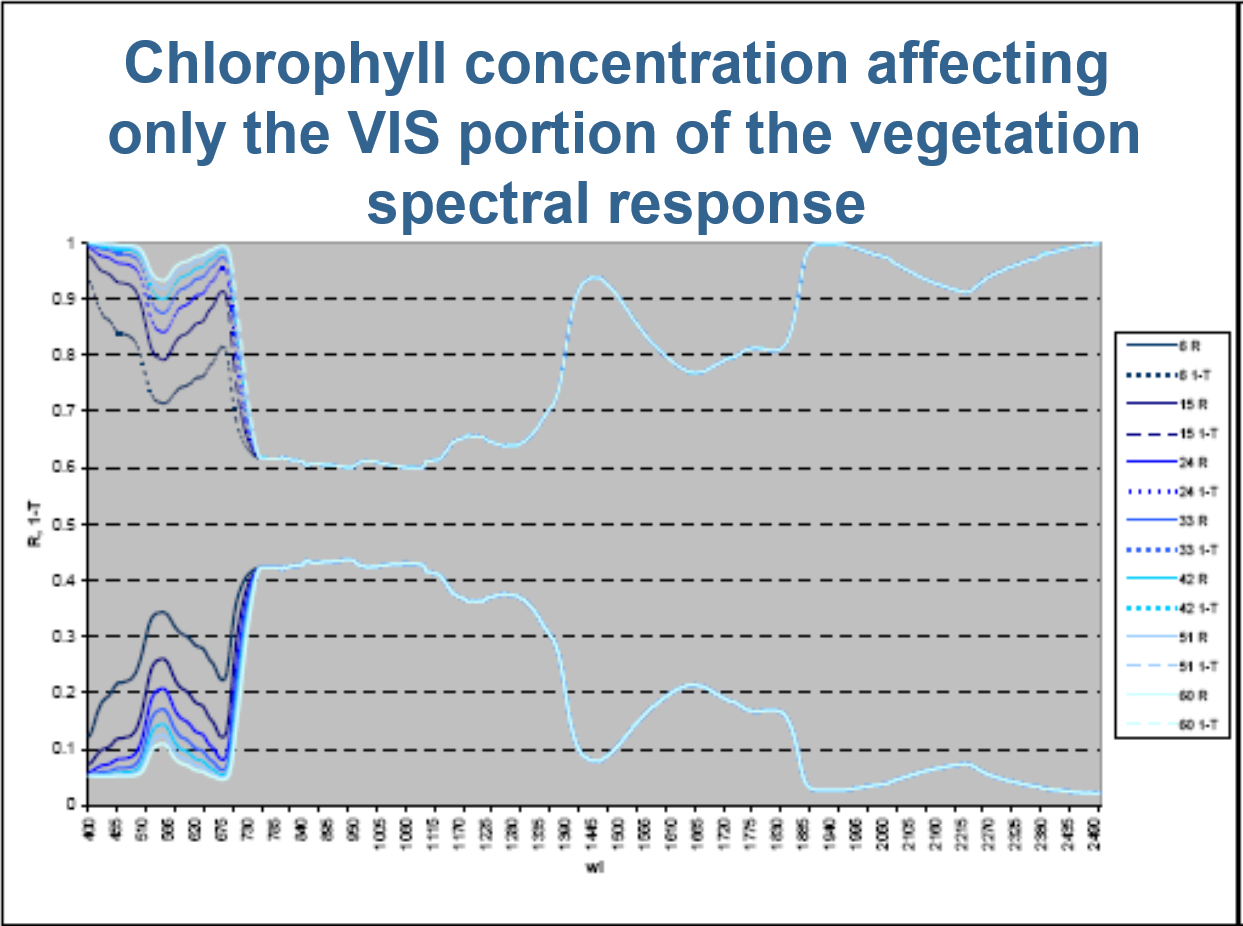 Total
Total Chlorophyll
Concentration
(\(\mu g \, cm^{-2}\))
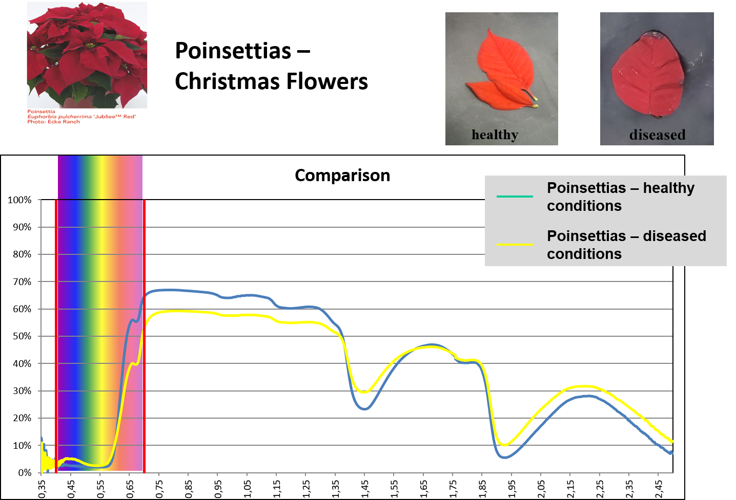
Monitoring vegetation disease
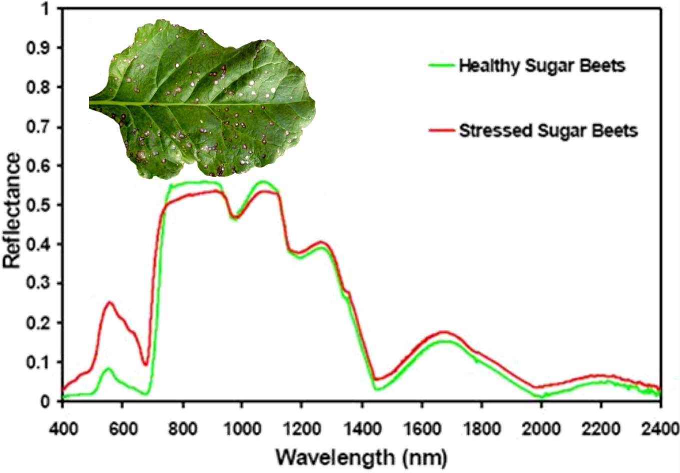
Spectral signatures of vegetation
\(\bbox[5px, border: 1px solid black]{\rho_\lambda + \alpha_\lambda + \Im_\lambda = 1}\)

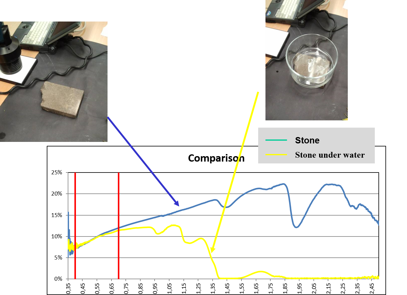
Spectral signatures of vegetation
(reflectance) and water (absorption)
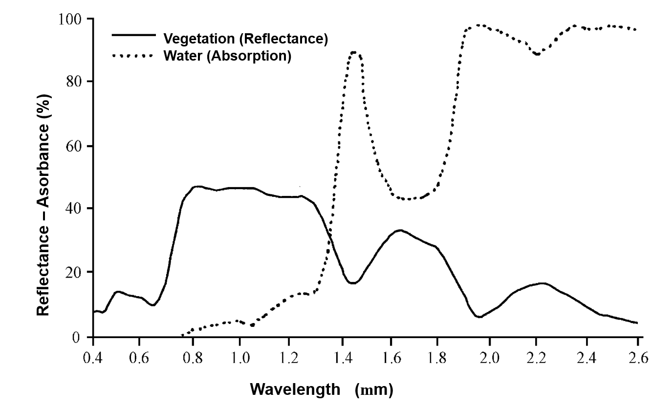
 Water depth
 [\(cm^{2}\)]
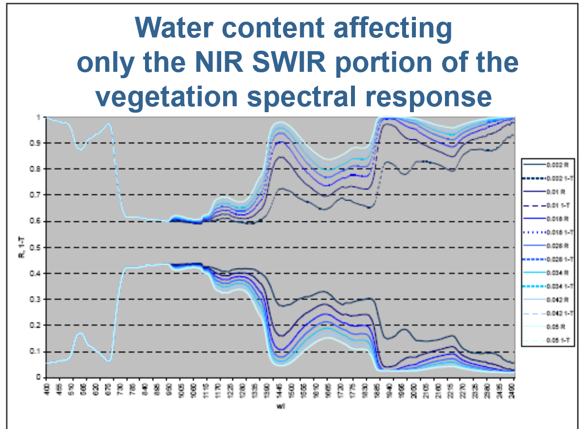
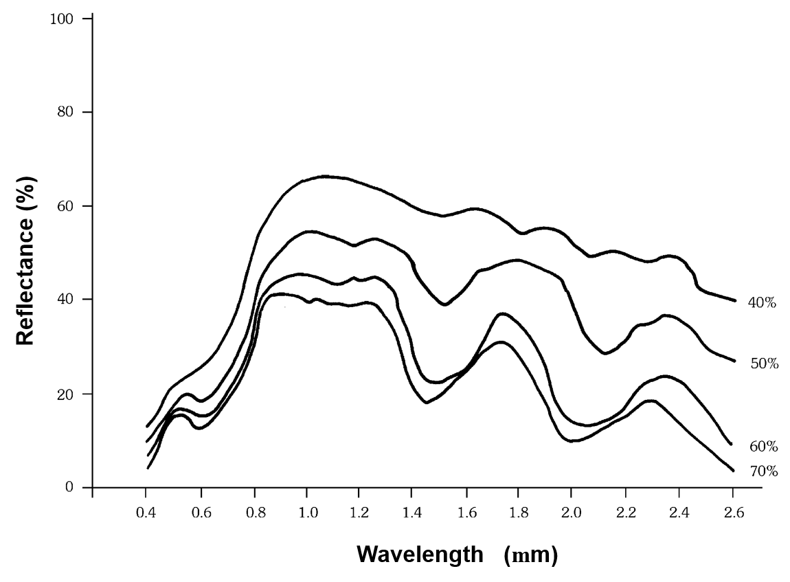
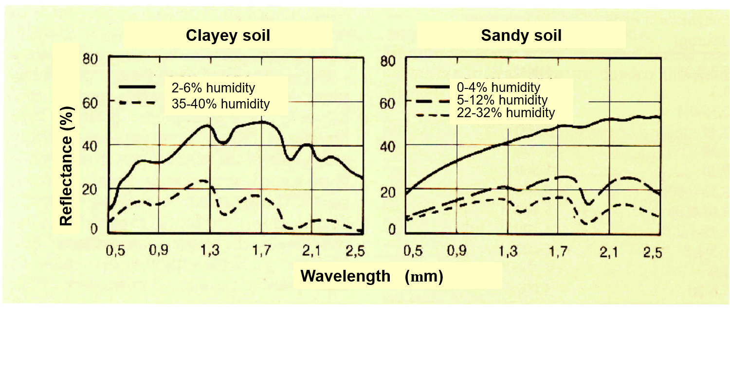
Spectral signatures of vegetation in
different condition of water stress
water content %
Measuring reflectances in the lab & in the field
(Field Spec ASD Spectrometer)
\(\bbox[15px, yellow]{NDVI = \frac{R_{NIR}-R_{VIS}}{R_{NIR} + R_{VIS}}}\)
NDVI
(Normalized Difference Vegetation Index)
on NDVI computation and applications
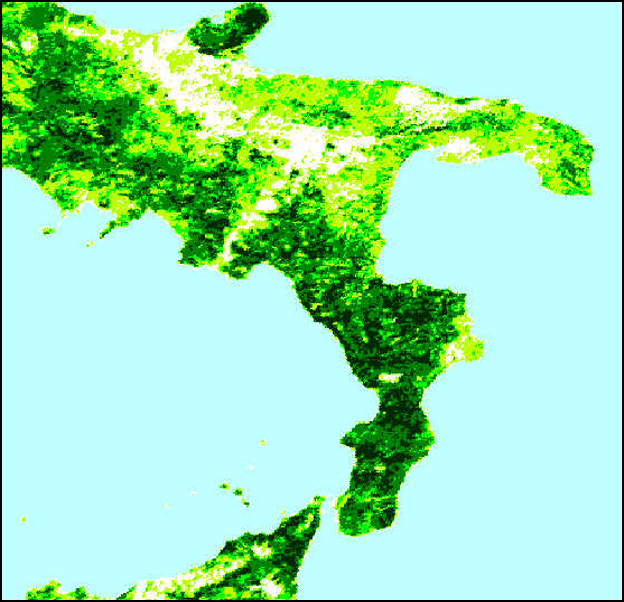
Example of NDVI reduction after fires
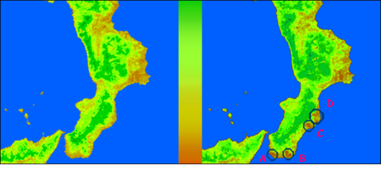
High
NDVI
Mid
Low
| Burned Areas | Wooded (ha) | Mixed Covers (ha) |
|---|---|---|
| A - Motta S.Giovanni e Melito di Porto Salvo | 141 | 3320 |
| B - Bova e Bova Marina | 3600 | 3300 |
| C - Grotteria e Roccella Ionica | 1150 | 2413 |
| D - Bivongi | 500 | 1000 |
Applications
Vegetation (Normalised Difference Vegetation Index)
\(\bbox[15px, yellow]{NDVI = \frac{R_{NIR}-R_{VIS}}{R_{NIR} + R_{VIS}}}\)
Problems?
Clouds, Atmospheric Effects, View Angle Effects
Solution?
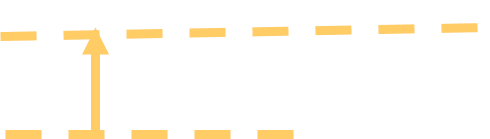
Maximum Value Composite (MVC)
 1
2
3
4
5
1
2
3
4
5
|
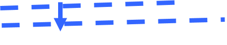
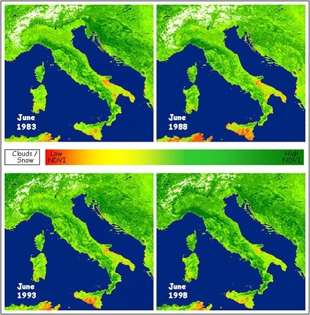
SEASONAL CHANGE AT REGIONAL SCALE

JUNE NOVEMBER

\(\bbox[15px, yellow]{NDVI = \frac{R_{NIR}-R_{VIS}}{R_{NIR} + R_{VIS}}}\)
Applications
Vegetation (Normalized Difference Vegetation Index
MONITORING OF DEFORESTATION
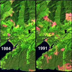
Applications
Vegetation (Normalized Difference Vegetation Index)
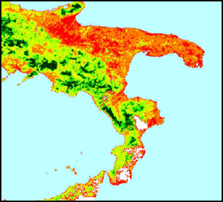
MONITORING OF DESERTIFICATION
 From the analysis
 of long (ten-year) time
series of NDVI
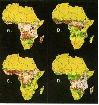
Seasonal change at continental scale
A. April 12-May 2, 1982;
B. B. July 5-25, '82;
C. Sept. 27-Oct. 17, '82;
D. Dec. 20, '82-Jan. 9, '83
\(\bbox[15px, yellow]{NDVI = \frac{R_{NIR}-R_{VIS}}{R_{NIR} + R_{VIS}}}\)
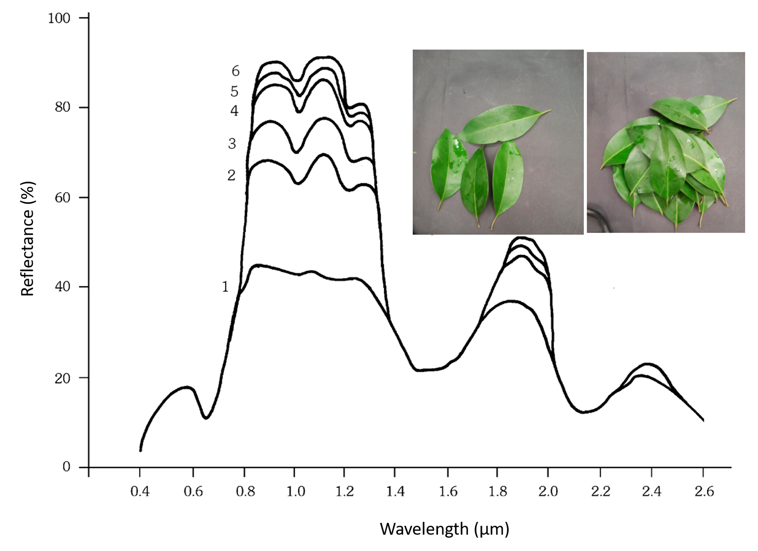
Spectral signatures of vegetation
\(\bbox[5px, border: 1px solid black]{\rho_\lambda + \alpha_\lambda + \Im_\lambda = 1}\)
high transmittance

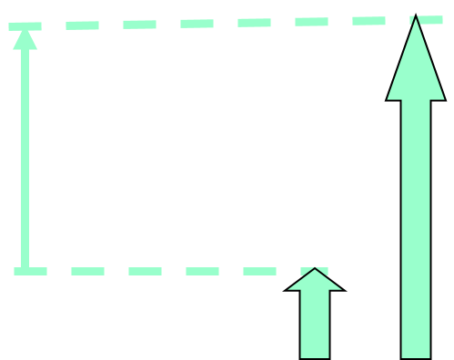
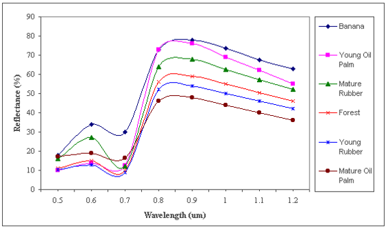
Dependence of reflected radiation on
vegetation density (Leaf Area Index)
Reflectance increases with vegetation
density where transmittance is higher
Spectral signatures of vegetation
(in reflectance)
Spectral signatures of soil, water,
vegetation (in reflectance)
Spectral signatures of different soils
(in reflectance)
Mixing
Atoms and molecule adsorb and emits at specific wavelength
atomic spectra molecular spectra
\(\frac{Ze^2}{r^2} = \frac{mv^2}{r} ~~~\Rightarrow~~~ r=\frac{Ze^2}{mv^2}\)
\(l_n = mvr_n = n\hbar ~~~\Rightarrow~~~ r_n = \frac{n^{2}\hbar^{2}}{me^2Z}\)
\(E=-\frac{Ze^2}{r}+\frac{1}{2}mv^2=-\frac{1}{2}\frac{Ze^2}{r}\)
\(E_n = -\frac{m_e e^4}{2\hbar^2} \cdot \left(\frac{1}{n^2}\right)Z^2\)
\(E_n = -\frac{m_e e^4}{2\hbar^2} \cdot \left(\frac{1}{n^2}\right)Z^2~~~\)energy of Bohr orbit
\(v_{jk} = R \cdot \left(\frac{1}{n_j^2}-\frac{1}{n_k^2}\right)Z^2\)
with
\(R=\)
Rydberg constant
\(~~~=\frac{2 \cdot \pi^2 \cdot m_e \cdot e^4}{h^3}\)
\(E_{mol}=E_{trasl}+E_{ele}+E_{vib}+E_{rot}\)
\(E_{trasl}~\propto~KT\)
\(E_{vib}^v = \hbar\sqrt{\frac{K}{\mu}}\left(V+\frac{1}{2}\right)~~~\Delta V = \pm 1\) with overtones
\(E_{rot}^J = \frac{\hbar^2}{2I}J(J+1)~~~\Delta J=\pm 1\)
\(v_{jk} = \frac{E_k-E_j}{h}\)
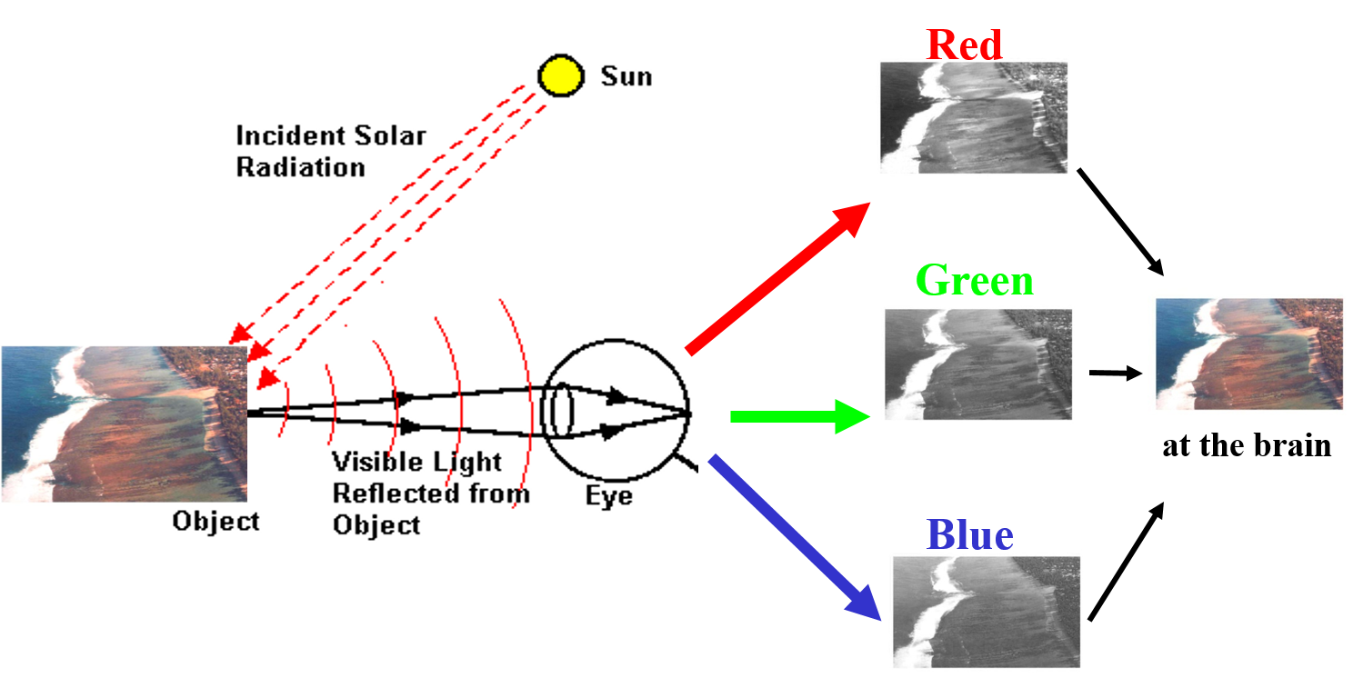
Basic principle of multi-spectral
remote sensing
- Every material emits, absorbs, transmits or reflects differently at different wavelengths, the em radiation, according to their chemical and physical characteristics
- The spectral response curve represents, in this sense, its spectral signature
- The availability of multi-spectral observations allows, in theory, to trace back to the chemical and physical characteristics of the material that has emitted, absorbed, transmitted or reflected measured em radiation.
From the lab
to the space.
From ground to space

beyond visible
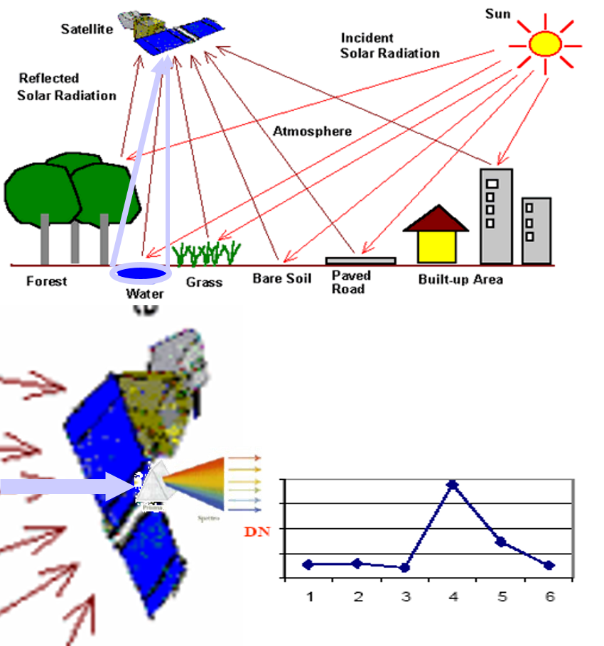

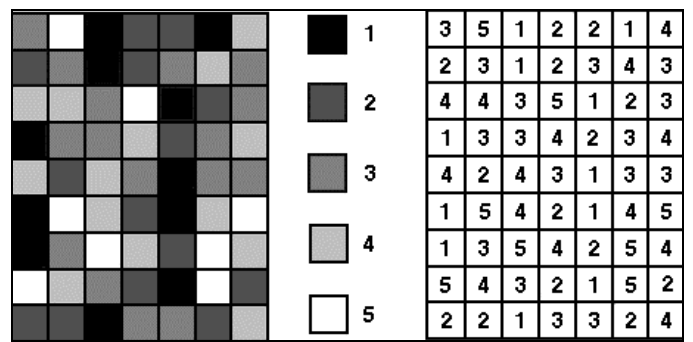
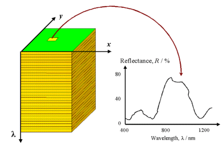
Multispectral digital image
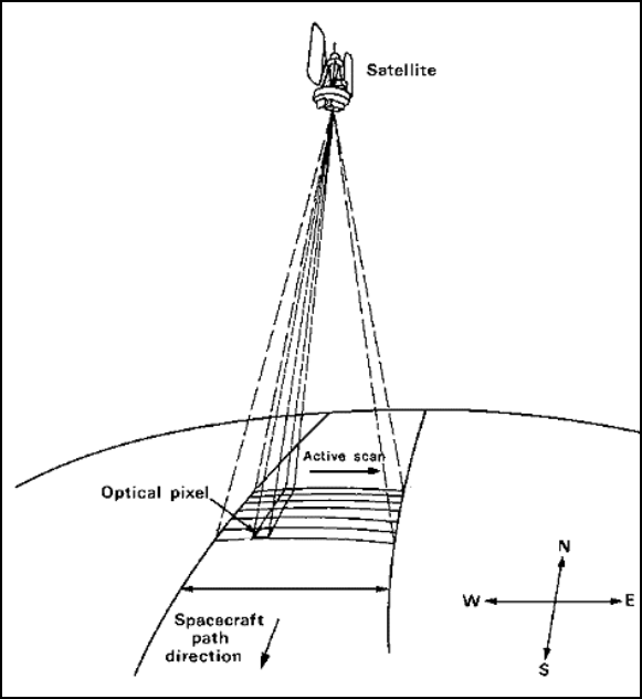
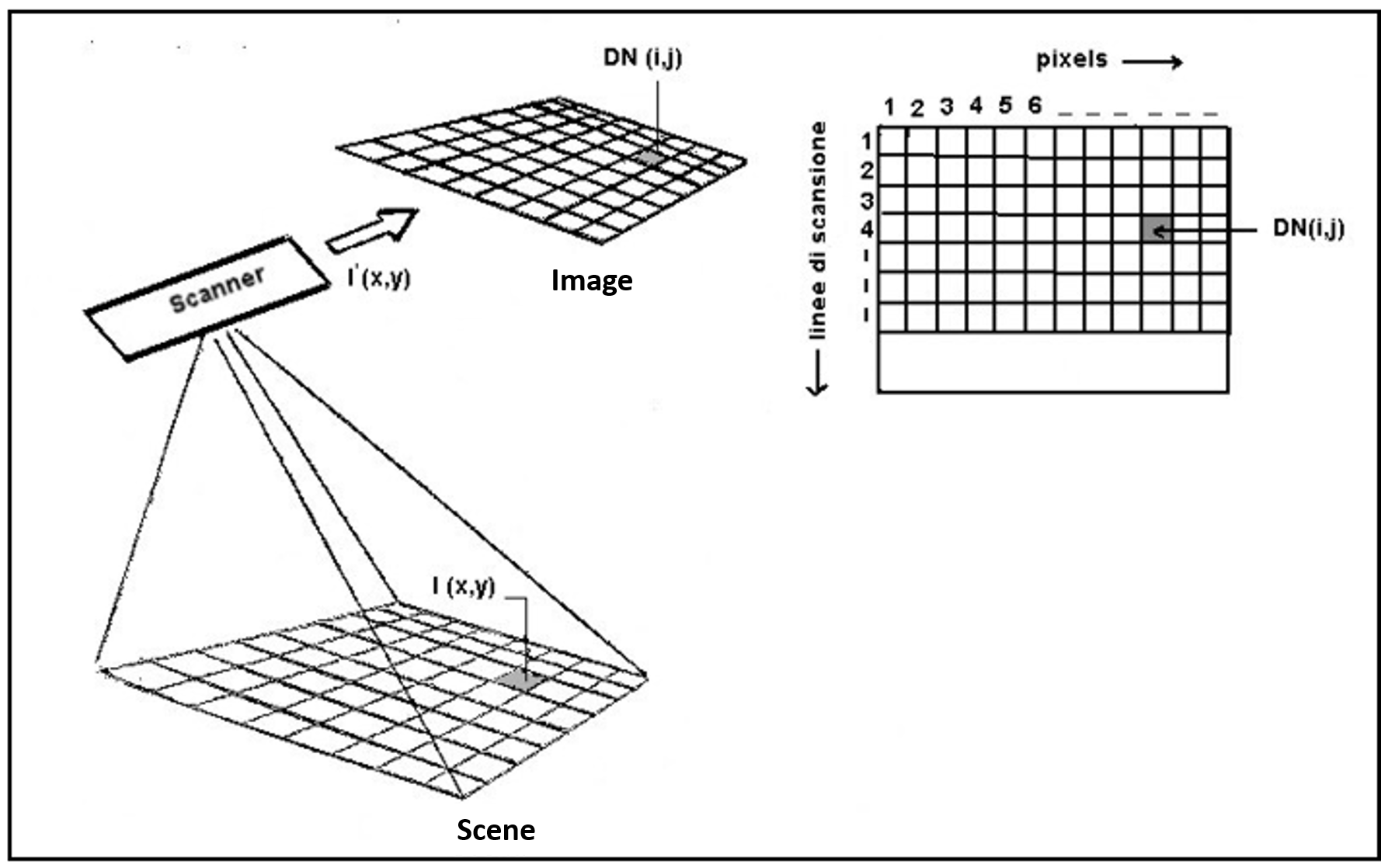
EO Sensors
Image systems and multispectral images
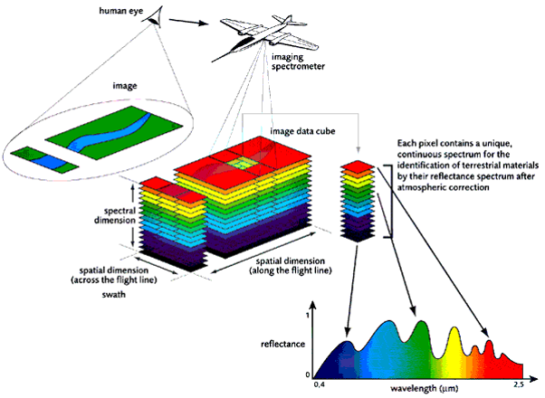
EO Sensors
Image systems and multispectral images
Spectral Signatures from
MODIS
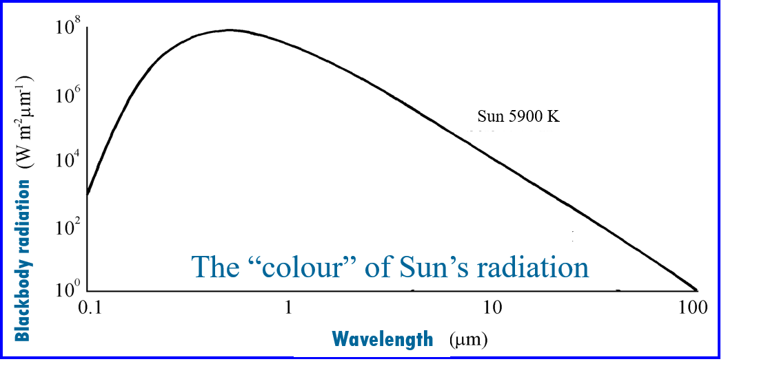
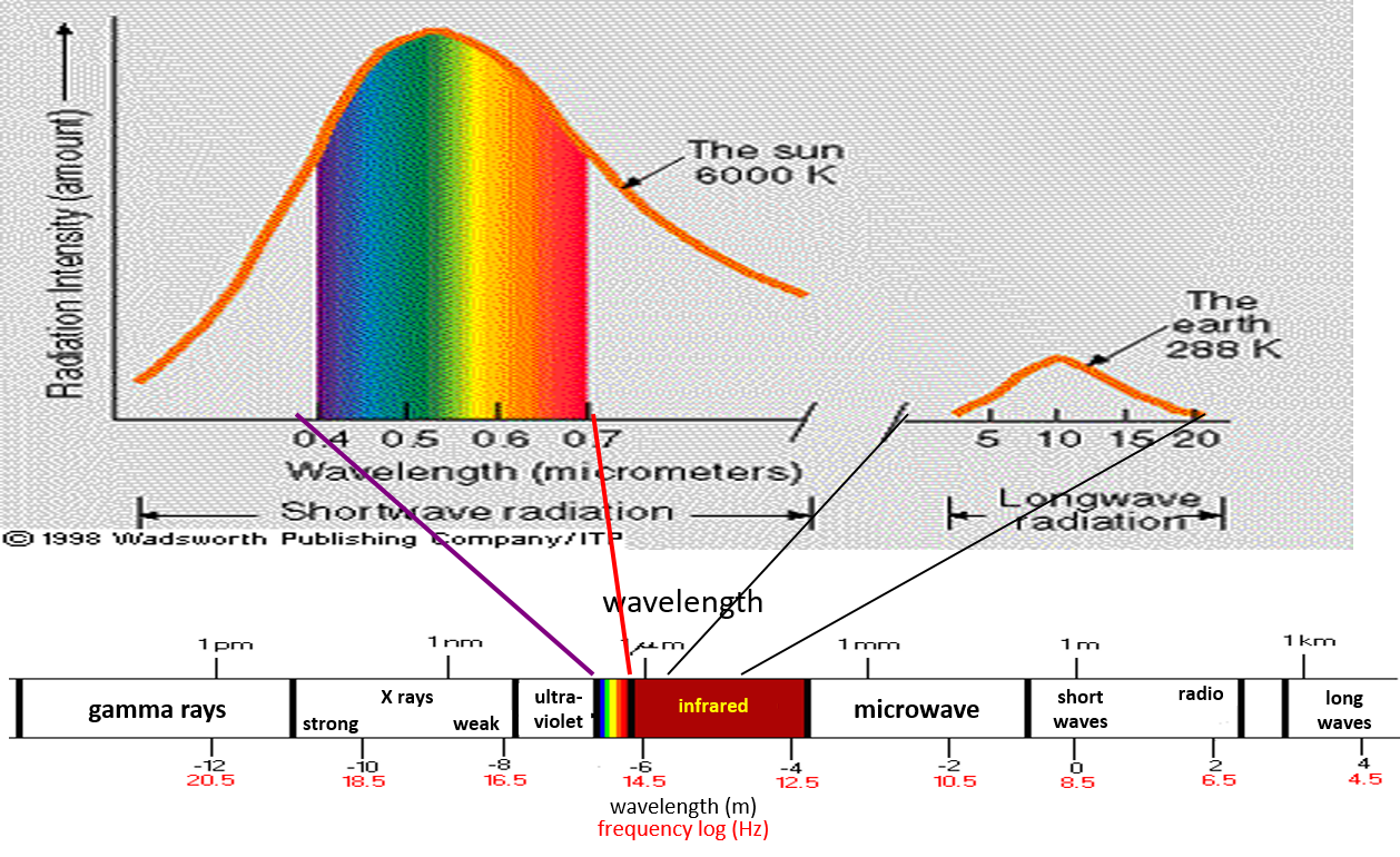
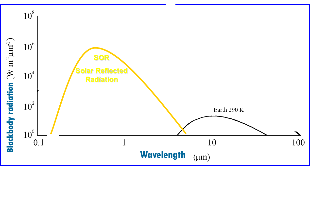
Natural sources of radiation for Earth Observation
The Sun(only daytime !)
Wien
\(\bbox[15px, border: 1px solid black]{\lambda_{MAX}=\frac{2898}{T(K)}\approx\frac{3000}{6000}=0,5\mu m}\)
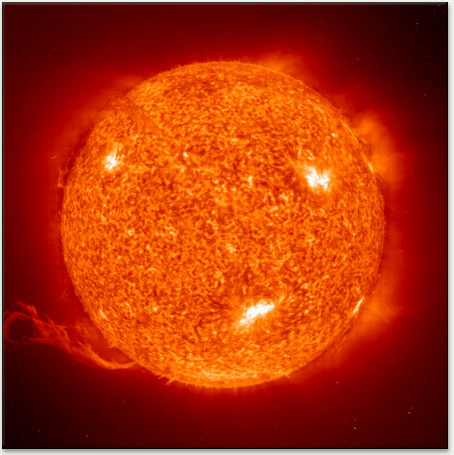 \(T\approx 6000K\)
Natural sources of radiation for Earth Observation
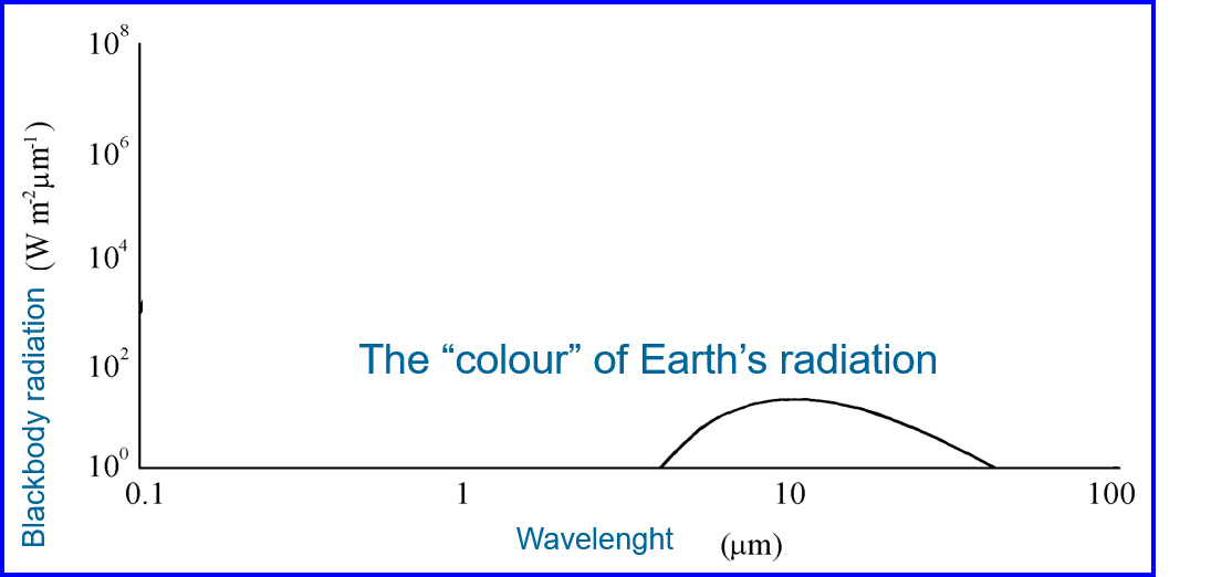
The Earth itself (day and night !)
Wien
\(\bbox[15px, border: 1px solid black]{\lambda_{MAX}=\frac{2898}{T(K)}\approx\frac{3000}{300}=10\mu m}\)
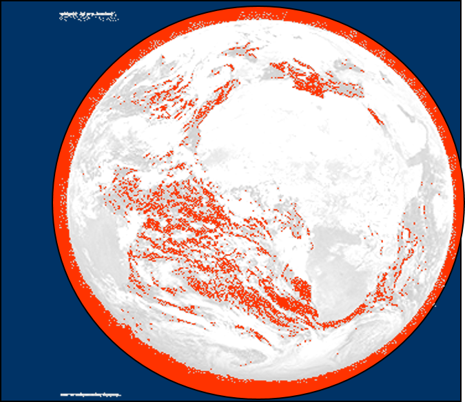 \(T\sim 300K\)
Solar and Terrestrial radiation
| Peak Wavelength | Max. Intensity | |
| Sun | \(0.5\) micrometers | \(7.35 \times 10^7 W/m^2\) |
| Earth | \(10\) micrometers | \(390 W/m^2\) |
Natural sources of radiation
actually available for EO
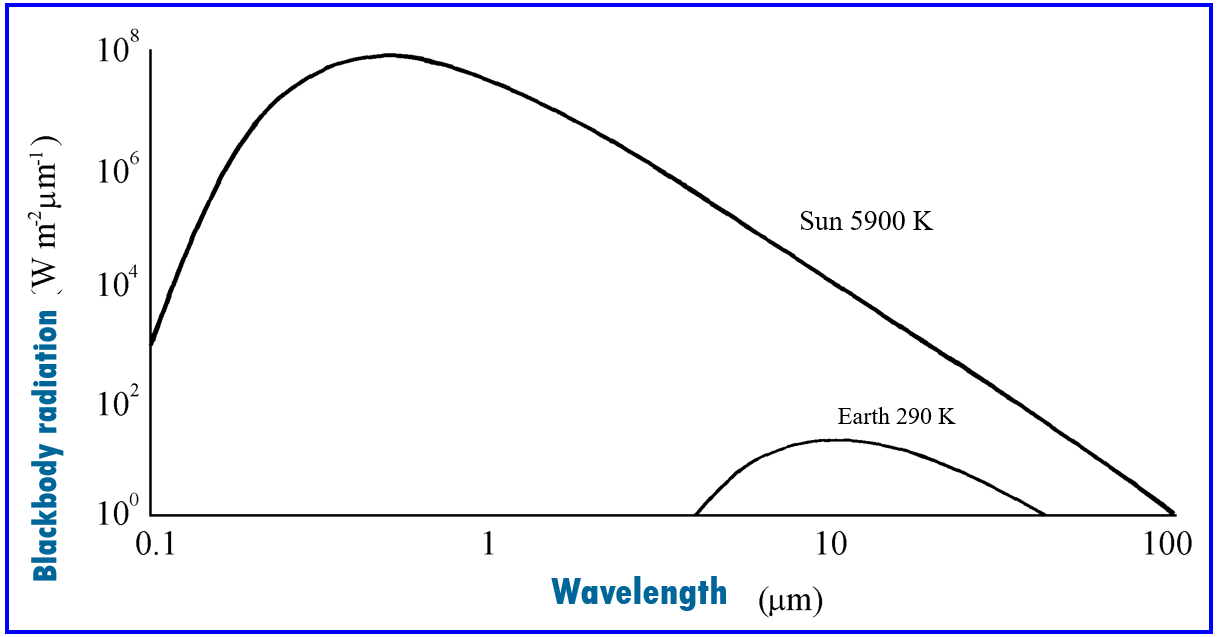
| Peak Wavelength | Max. Intensity | |
| Sun | \(0.5\) micrometers | \(7.35 \times 10^7 W/m^2\) |
| Earth | \(10\) micrometers | \(390 W/m^2\) |
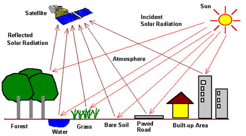
Passive Earth Observing Techniques
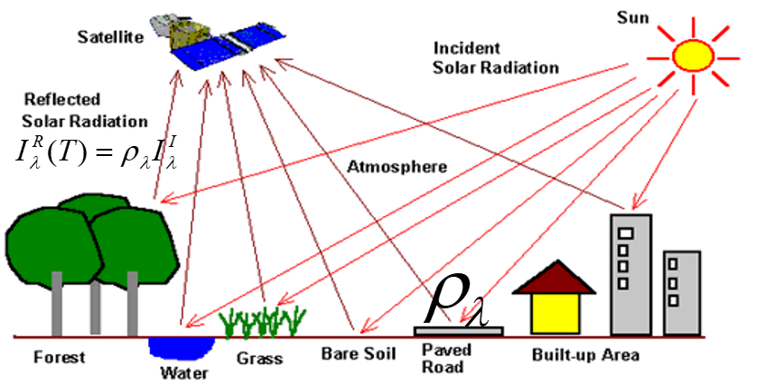
Natural source of
radiation (Sun) different
from the target
Diagnostic parameter:
\(\rho_\lambda\)
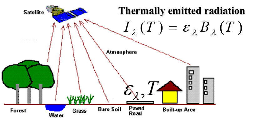
Natural source of
radiation (Earth)
coincident with the target
Diagnostic parameters:
\(\epsilon_\lambda, T\)
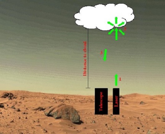
Active Earth Observing Techniques
The signal is generated
by the observation
system itself
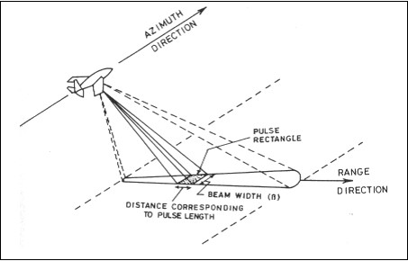
Diagnostic Parameter
\(I_\lambda^{back} \propto\) roughness
\(\frac{c\Delta t}{2}=d=\) distance
e.g. SAR (Synthetic
Aperture Radar)
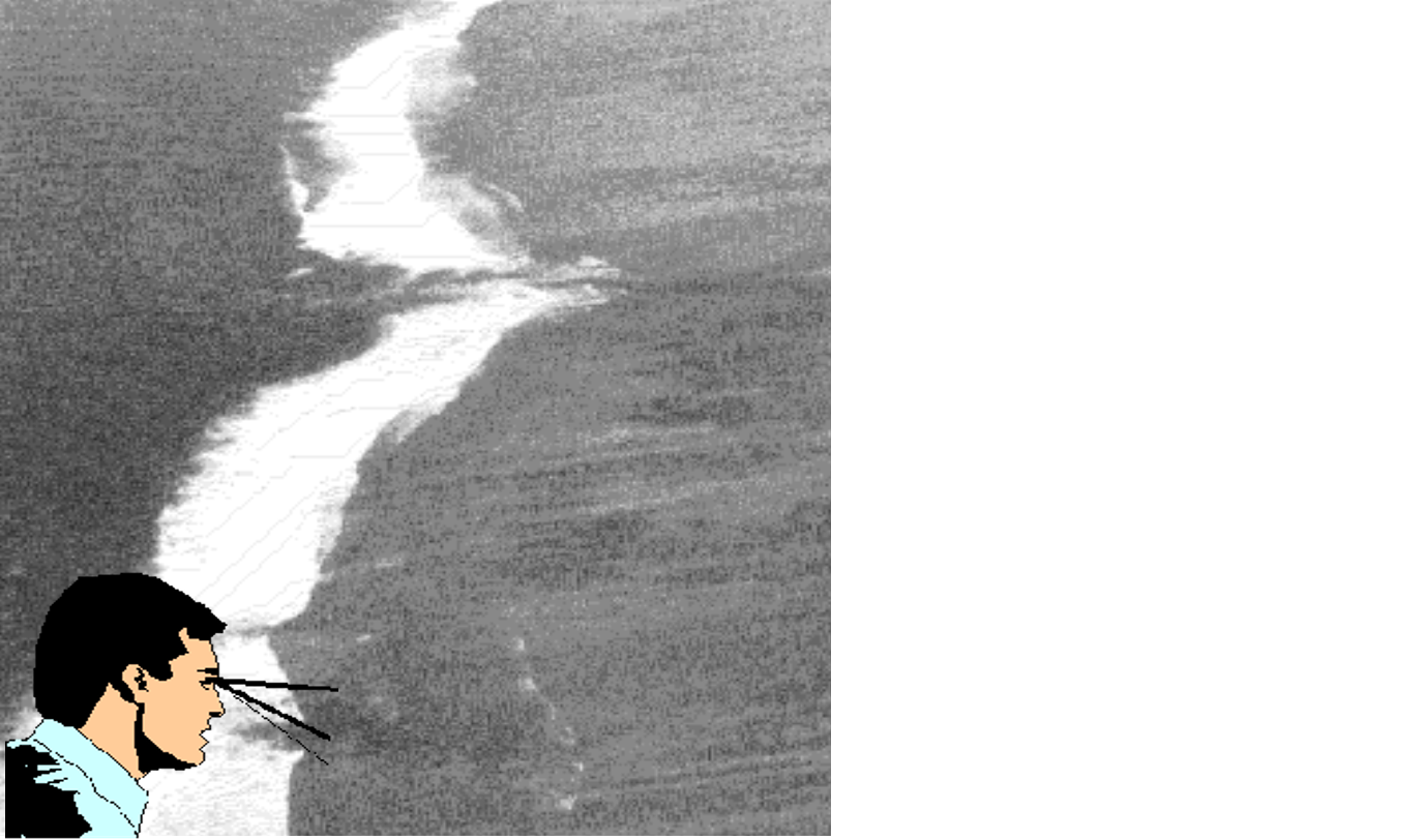
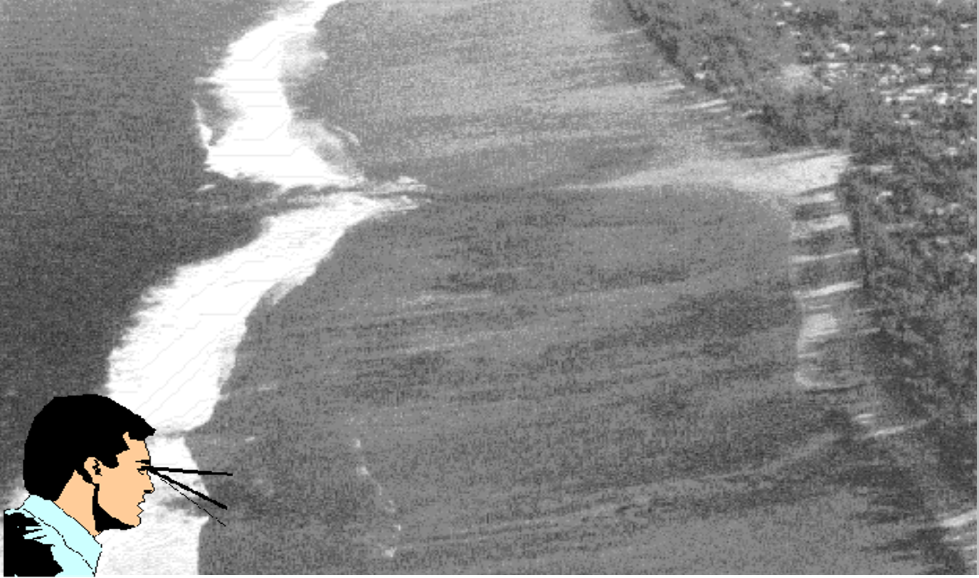
Different spectral region different capabilities
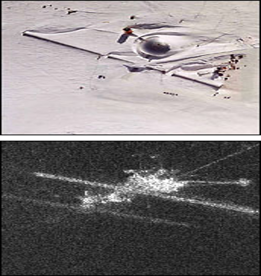
This pair of images demonstrates some of the differences between passive and active sensors. The top image is an aerial photograph (which records reflected light) of Amundsen-Scott Station, a research facility built on the South Pole. The bottom image is the same area, at approximately the same scale and orientation, from RADARSAT. RADARSAT is an active remote sensing instrument. Microwaves are generated by the sensor, reflected from the Earth's surface and back to the sensor. The radar image reveals an abandoned cluster of buildings (to the lower left of the bright dome) that are now buried under Antarctic ice. (RADARSAT image courtesy Canadian Space Agency)
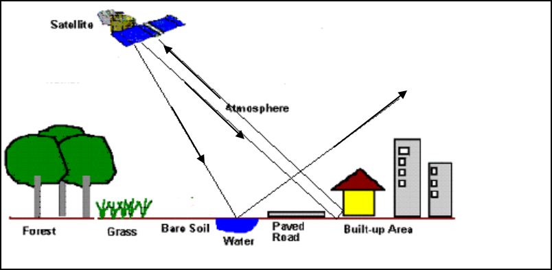
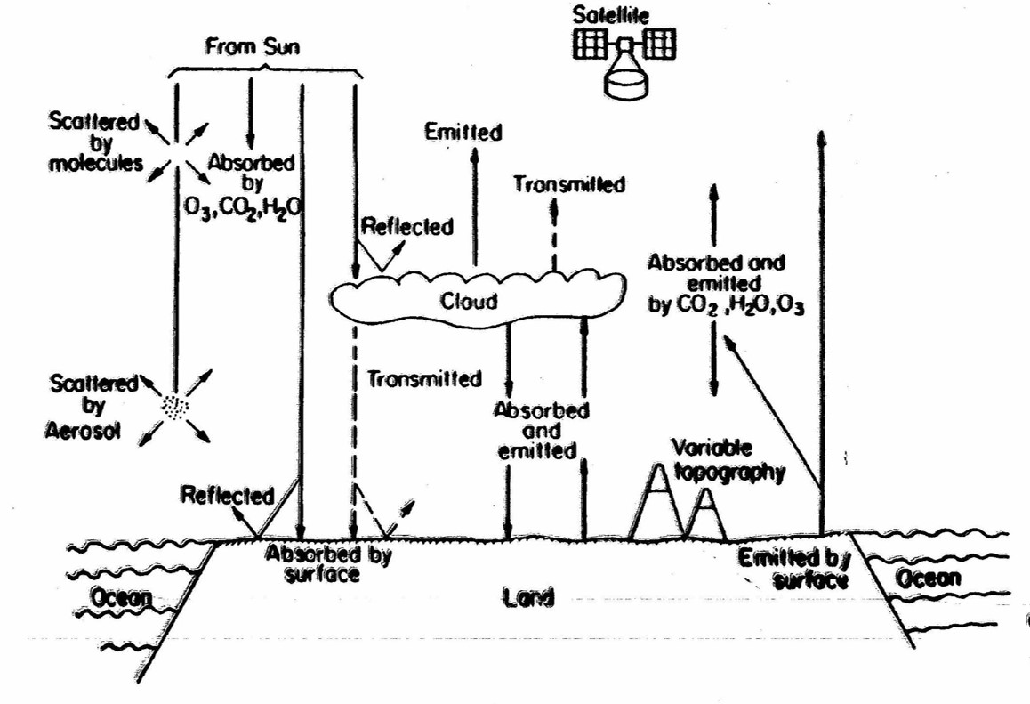
Atoms and molecule in atmosphere interact
selectively with (modifying) the radiation leaving
Earth surface and directed toward the sensor.
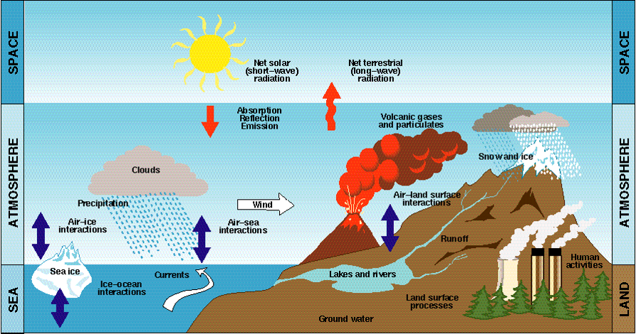
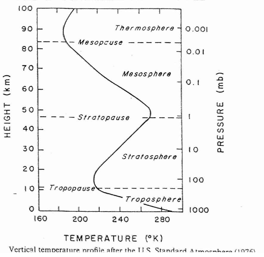
Chemical-physical properties of
atmosphere: temperature profile
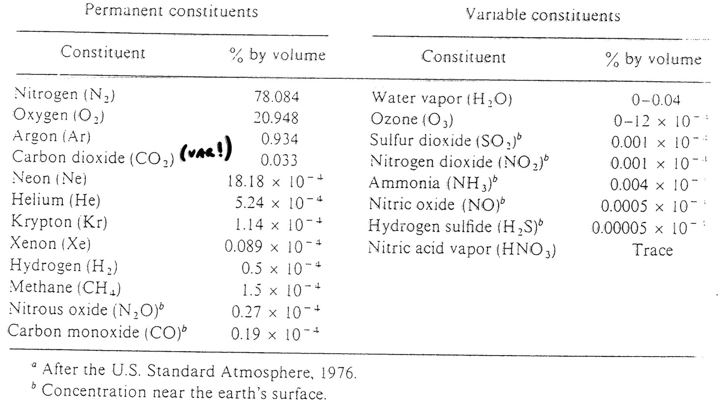
Chemical composition
Chemical composition of
atmosphere
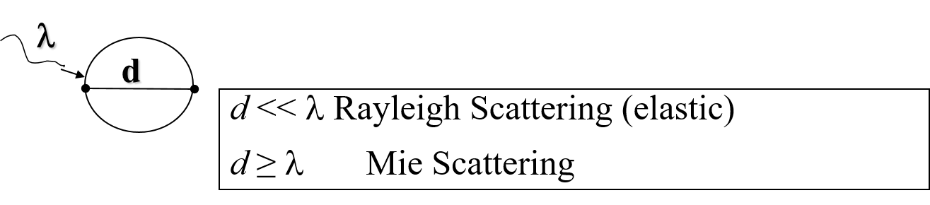
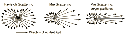
Scattering in the atmosphere
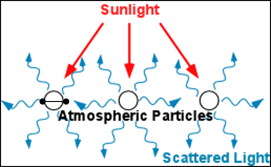
In general we can have scattering for whatever
wavelength \(0 < \lambda < \infty \)
in the atmosphere we have scattering from particle
having dimension like:
\(10^{-8} < d < 1 \quad cm\)
\( [X~rays]~~~~~[microwaves]\)
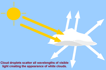
What about clouds?
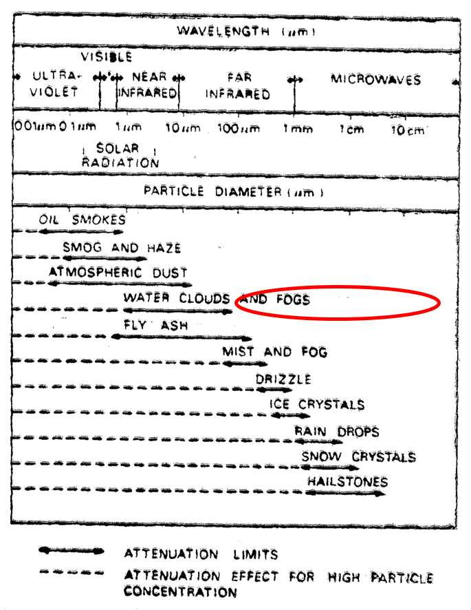
Attenuation to radiation of
different wavelengths by
common atmospheric constituents
and other particles (Source:
Tomlinson 1972)
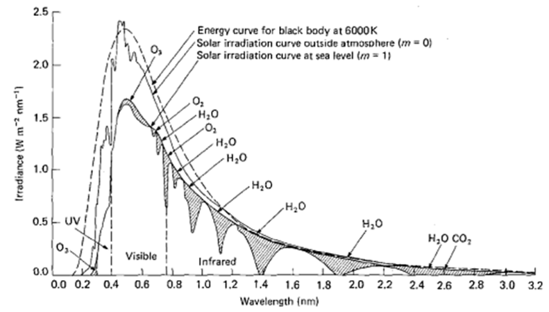
Extinction of solar radiation
in the atmosphere
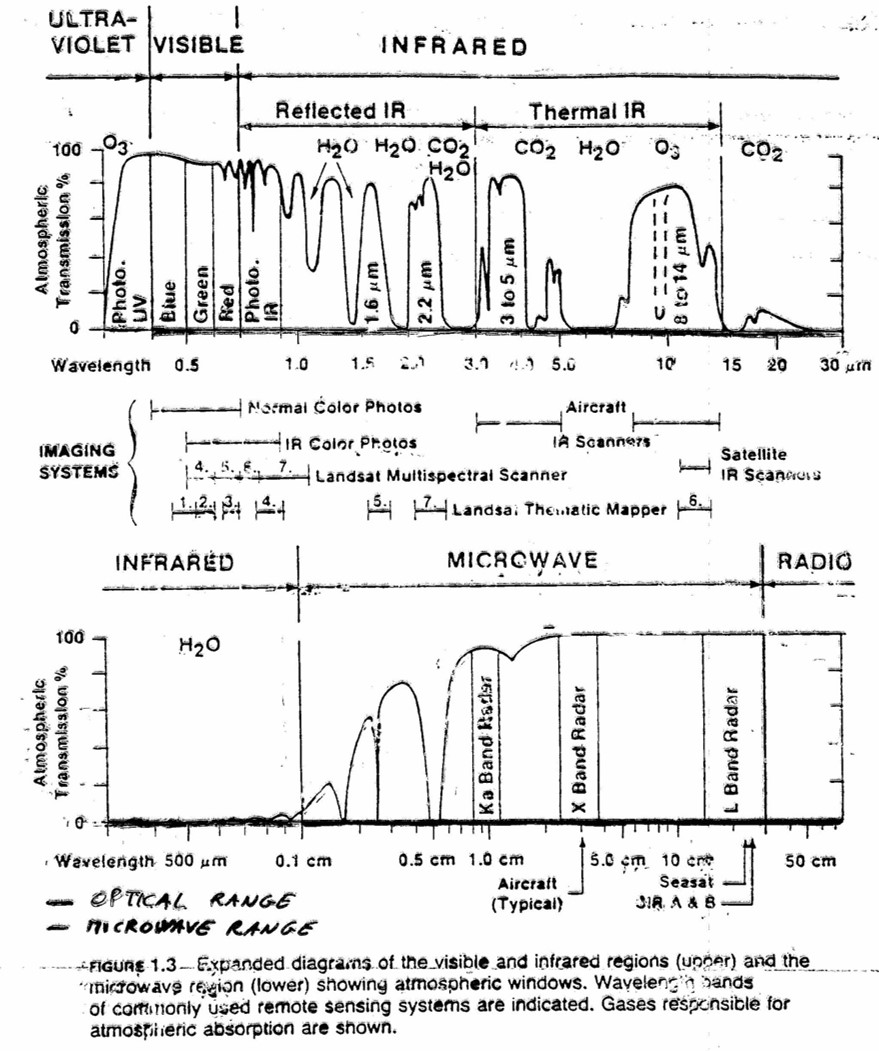 Atmospheric
 Transmittance and
atmospheric windows
LANDSAT-TM all bands in atmospheric windows !
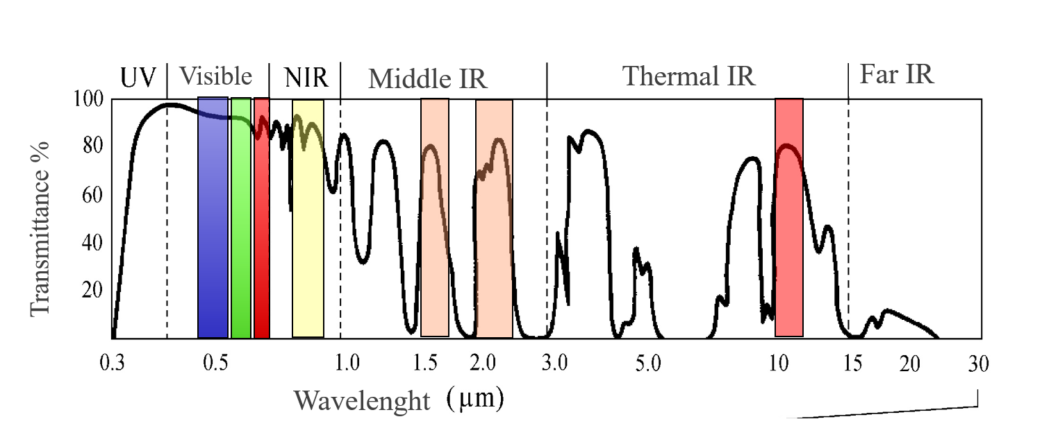
AVHRR:
all bands in atmospheric windows !
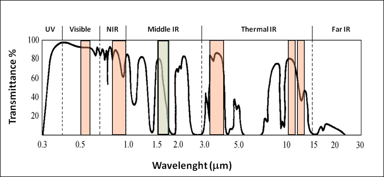
with corresponding atmospheric transmittance
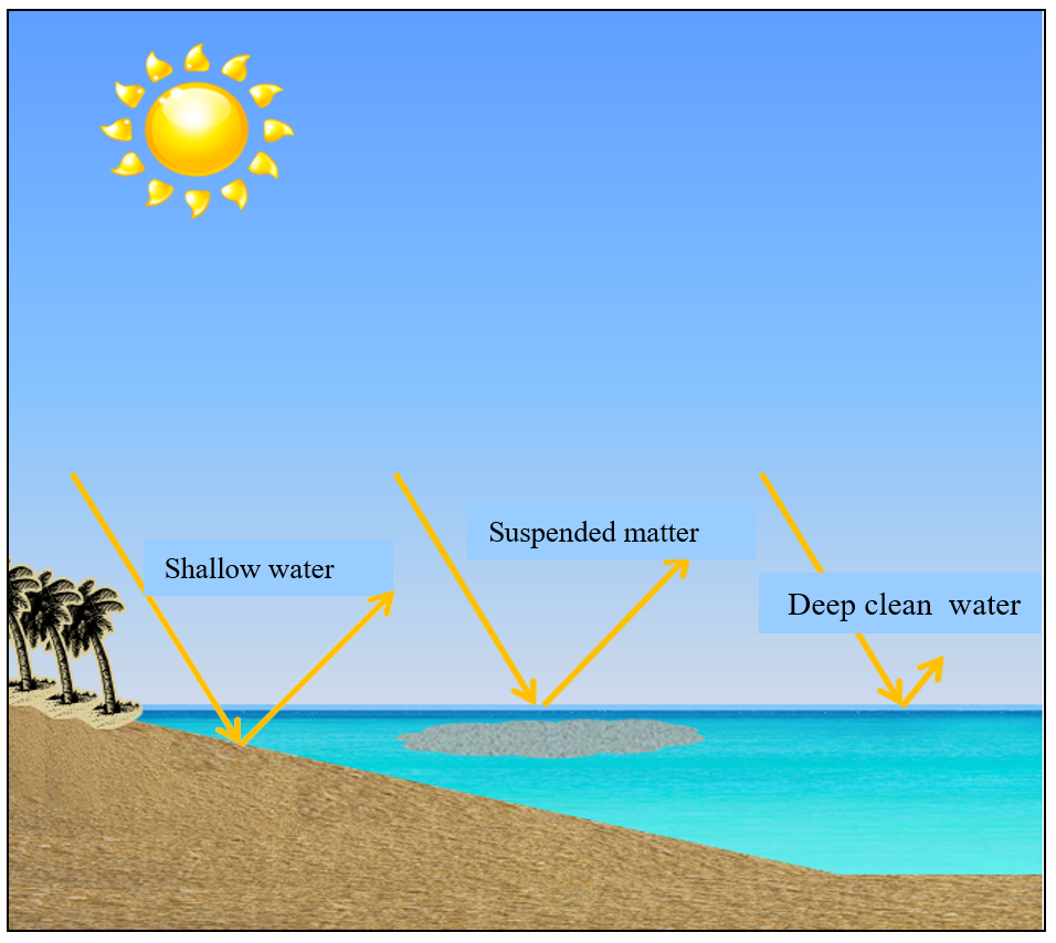
Penetration of e.m. radiation into the matter
Penetration of em radiation in a medium
with complex refractive index
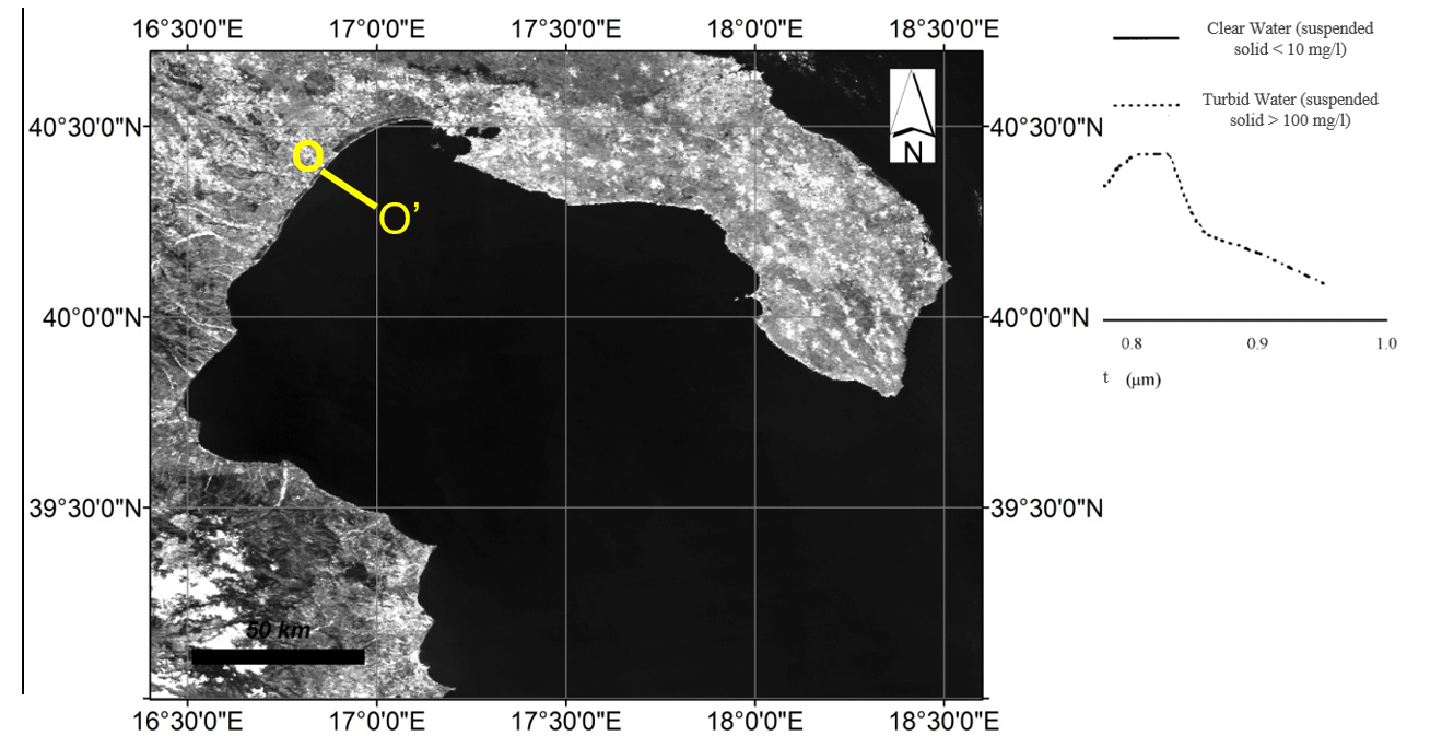
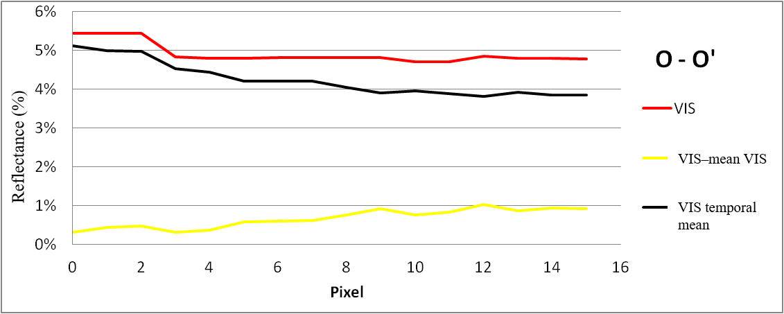
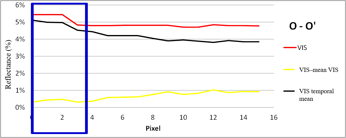
sediments or shallow water?
Sediments or shallow water ?
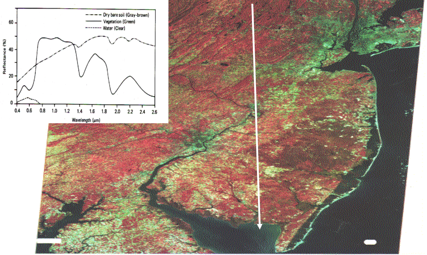
LANDSAT -MSS
Band 4 = Blue Band 5 = Green Band 7 = Red
Multitemporal approach (Di Polito et al., 2016)
What about clouds?
cloud mask
Reference list
R. P. Gupta Remote Sensing Geology, Springer & Verlag, (1991).
W.G. Rees, Physical Principles of Remote Sensing, Cambridge University Press (1990)
Il telerilevamento da aereo e da satellite libro Brivio P. A. (cur.) Lechi G. M. (cur.) Zilioli E. (cur.) edizioni Delfino Carlo Editore collana Scienza & tecnica , 1992