Delineating agricultural parcels using deep learning
Learning objectives
The goal of this training is to teach you how to perform parcel delineation covering all aspects involved: the machine learning part, the computing part as well as what to keep in mind when prepping your data.
-
At the end of this training, you will:
- Know how a U-Net works and why it was developed
- Know about recent developments in distributed computing and why they are necessary
- Be familiar with basic and more complex operations in openEO
- Be able to do inference of pre-trained U-Net models yourself
- Be able to do delineate agricultural parcels
List of abbreviations
Table of contents
- Introduction
- Field delineation: choosing a model
- History of edge detection
- U-Net
- Pre- and postprocessing
- Field delineation: choosing a platform
- Introduction to openEO
- openEO workflows
- openEO in practice
- Let's start coding: demo notebooks
Table of contents
- Introduction
- Field delineation: choosing a model
- History of edge detection
- U-Net
- Pre- and postprocessing
- Field delineation: choosing a platform
- Introduction to openEO
- openEO workflows
- openEO in practice
- Let's start coding: demo notebooks
Introduction
Importance of field delineation:
- decision making and planning of ministries and private sector
- facilitation of land registration and acquisition of land use rights for smallholder farmers
- estimate subsidies
- scientific purposes (climate modeling)
- regulate water rights
- can improve classification results in other EO applications (e.g. crop classification)
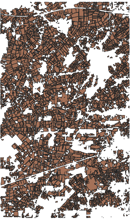
Field delineation
Advanced use case that can be solved using instance segmentation
Table of contents
- Introduction
- Field delineation: choosing a model
- History of edge detection
- U-Net
- Pre- and postprocessing
- Field delineation: choosing a platform
- Introduction to openEO
- openEO workflows
- openEO in practice
- Let's start coding: demo notebooks
Pre-DL edge detection methods
- Roberts cross
- Sobel
- Prewitt
- Laplacian
- Canny
Filters, but... small number and not trainable
Rise of DL: CNN
When thinking of filters and trainable parameters, we think of...
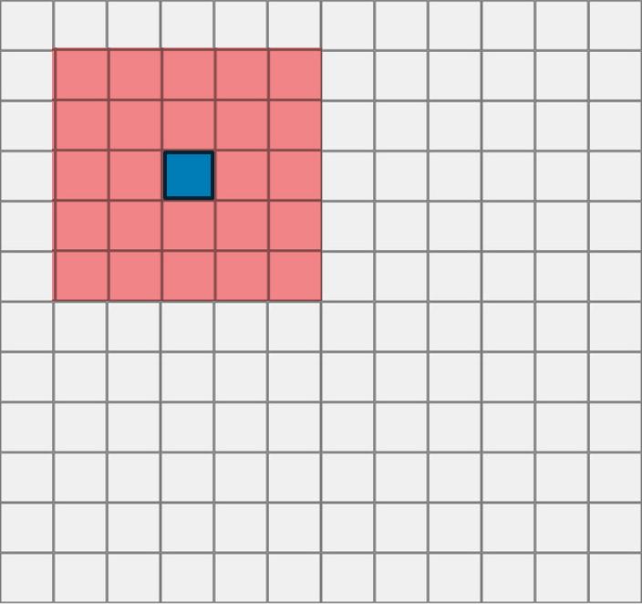
Convolution

Max pooling

More complex CNN's
Still are composites of these basic operations
What.. but where?
Standard CNN's can be used to predict what is in the image, but not where in the image it isCiresan et al. 2012
- Slow
- Small receptive field
Works by doing inference using a CNN (i.e., classifying "what") for every pixel in the image (hence getting an idea about the "where")
Outperformed by large margin competition on ISBI 2012 segmentation challenge, but...
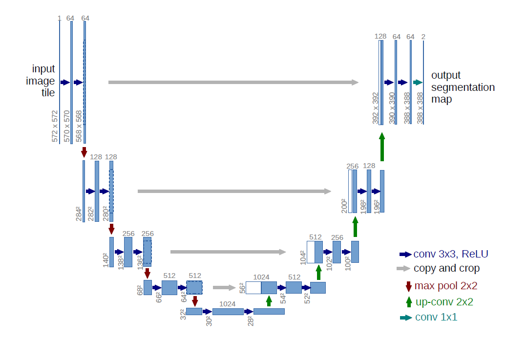
The solution: U-Net
- Based on paper: https://arxiv.org/pdf/1505.04597.pdf
- Original code based on caffe and available as well
- Winner of ISBI cell tracking challenge 2015
The authors succesfully attempted to calculate both the "what" and the "where" in one single neural network by adding an upconvolution path to a standard CNN recreate original image dimensions
U-Net architecture
Transposed convolution

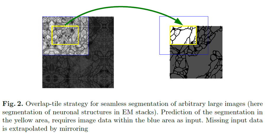
Overlap strategy: mirroring
U-Net implementation in this demo
-
Adaptations made to original U-Net:
- Use of sigmoid instead of softmax with two classes
- Same padding instead of valid padding (=no padding) > no need for cropping
- Input / output dimensions are different (128x128)
- Added batch normalization
This U-Net implementation
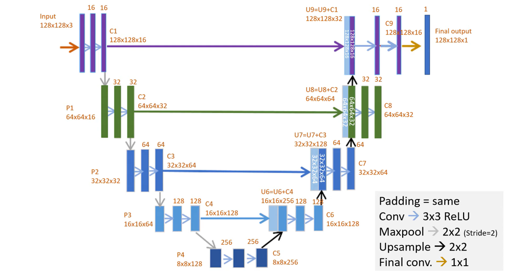
Table of contents
- Introduction
- Field delineation: choosing a model
- History of edge detection
- U-Net
- Pre- and postprocessing
- Field delineation: choosing a platform
- Introduction to openEO
- openEO workflows
- openEO in practice
- Let's start coding: demo notebooks
Pre- and postprocessing
Remember, U-Net takes 3 * height * width input, in which 3 is generally RGB
-
EO data is more complex:
- More bands than just RGB
- An added dimension: temporal
Therefore we use NDVI to compress the band dimension and pass 3 different temporal snapshots as input
Preprocessing
The temporal NDVI snapshots are chosen based on the amount of cloud-affected pixels they contain.
Wrt preprocessing, the NDVI data is clamped as well as rescaled.
Postprocessing

Also, U-Net does not do instance segmentation; it is a semantic segmentation algorithm.
-
Therefore, we:
- take the original continuous sigmoid output of the network
- apply an extra post-processing step of calculating edges on the segmentation output using traditional filters
- perform rag boundary analysis to convert them to instance segments
RAG
A Region Adjacency Graph (RAG) is composed of nodes/vertices representing regions and edges, and their respective adjacency determined by weights (rag_boundary). Different regions within a RAG can be merged based on their weights (cut_threshold).
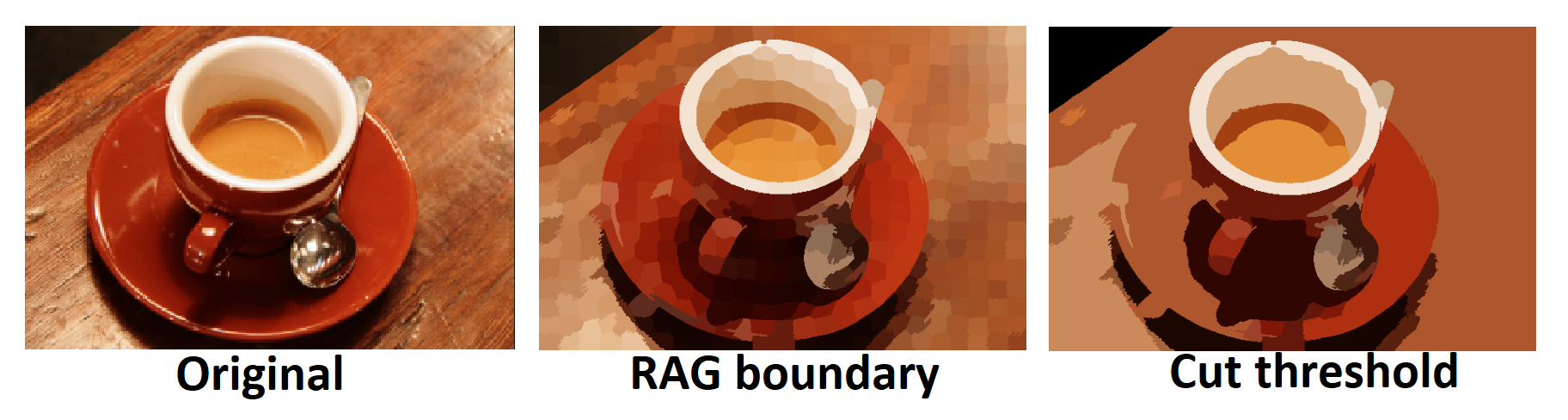
Table of contents
- Introduction
- Field delineation: choosing a model
- History of edge detection
- U-Net
- Pre- and postprocessing
- Field delineation: choosing a platform
- Introduction to openEO
- openEO workflows
- openEO in practice
- Let's start coding: demo notebooks
Traditional workflow

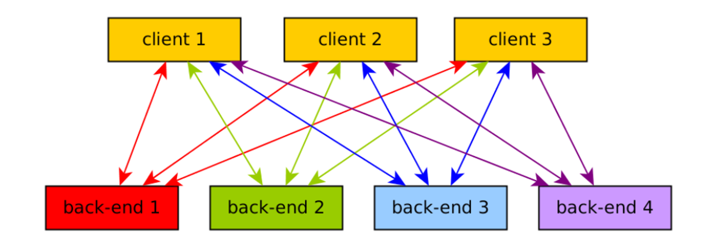
Cloud providers
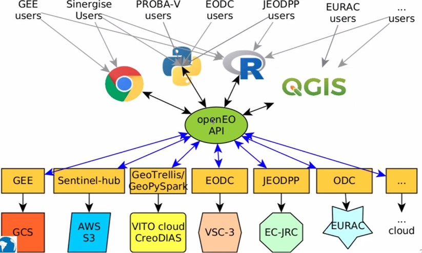
Solution: openEO
openEO develops an open application programming interface (API) that connects clients like R, Python and JavaScript to big Earth observation cloud back-ends in a simple and unified way.
Website of openEO platform
Solution: openEO
Various backends can be accessed through openEO using same client side syntax
openEO: data harmonization

openEO: inner workings
Client operations are transformed to JSON in a format called "process graphs", and sent to the various backends to be interpreted and executed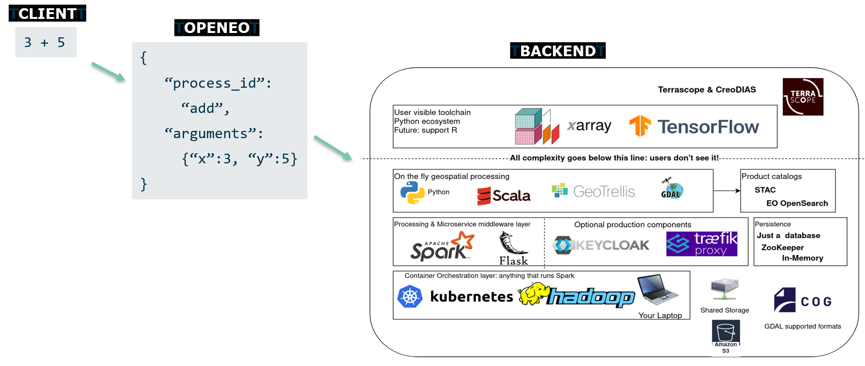
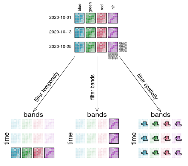
openEO: datacubes
Collections are represented as datacubes. Datacubes are multidimensional arrays with one or more spatial or temporal dimension(s) Datacubes
Table of contents
- Introduction
- Field delineation: choosing a model
- History of edge detection
- U-Net
- Pre- and postprocessing
- Field delineation: choosing a platform
- Introduction to openEO
- openEO workflows
- openEO in practice
- Let's start coding: demo notebooks
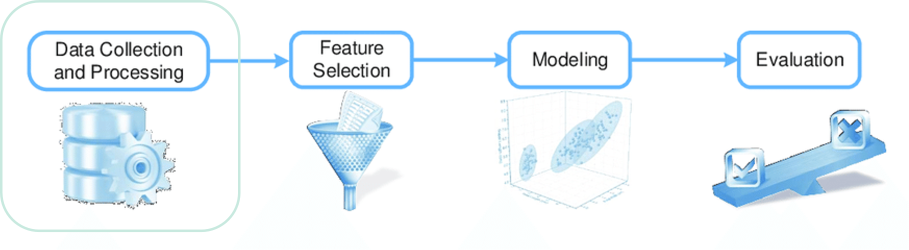
ML workflow: data collection
Available collections
76 collections available, a.o.:
Sentinel 1-2-3-5p
Landsat 4-5-7-8
Copernicus DEM
PROBA-V
MODIS
Copernicus Global Land
ECMWF Agera5
Coming up:
WorldCover Landcover
EEA Phenology
Commercial data
Additional Euro Datacube collections
ML workflow: feature engineering

Feature engineering operations
- Rescaling
- Resampling
- Applying functions along the temporal or band dimension
- Calculating indices
- Feature sampling
ML workflow: modeling & evaluation

Modeling outside of openEO
Generally, modeling is done outside of openEO. The workflow then looks like this:- Load a collection, calculate features
- Extract the features into points for which you have reference data using filter_spatial
- Train a model locally in your own environment, own GPU's, etc.
- Apply your model using a UDF (see next slide)
Click here for the documentation on feature sampling using filter_spatial. Click here for a code example of sampling using filter_spatial and applying model using UDF.
UDFs: User Defined Functions
Writing custom code that can be executed on a backend
- Applying a process to each pixel: apply
- Applying a process to all pixels along a dimension, without changing cardinality: apply_dimension
- Reducing values along a dimension: reduce_dimension
- Applying a process to all pixels in a multidimensional neighborhood: apply_neighborhood
Used in four different situations:
Click here for more information on UDFs.
Modeling in openEO
Some basic modeling is also supported within openEO, but at the moment only Random Forest and Catboost. However, at the moment automated tuning methods such as GridSearch or RandomSearch are not supported, so it is likely still faster to use previous method depending on your use case.Click here for an example code using our native Random Forest.
Click here for the documentation on native ML functionality.
ML workflow: inference

Inference
-
If you generated a model outside of openEO, you will do inference using a UDF. Some examples:
- UDF documentation
- In-line code example
- Separate python files code example
-
If you generated a model inside of openEO, you will do inference using predict_random_forest or predict_catboost.
- Documentation
- Example code
Summary

Table of contents
- Introduction
- Field delineation: choosing a model
- History of edge detection
- U-Net
- Pre- and postprocessing
- Field delineation: choosing a platform
- Introduction to openEO
- openEO workflows
- openEO in practice
- Let's start coding: demo notebooks
Documentation
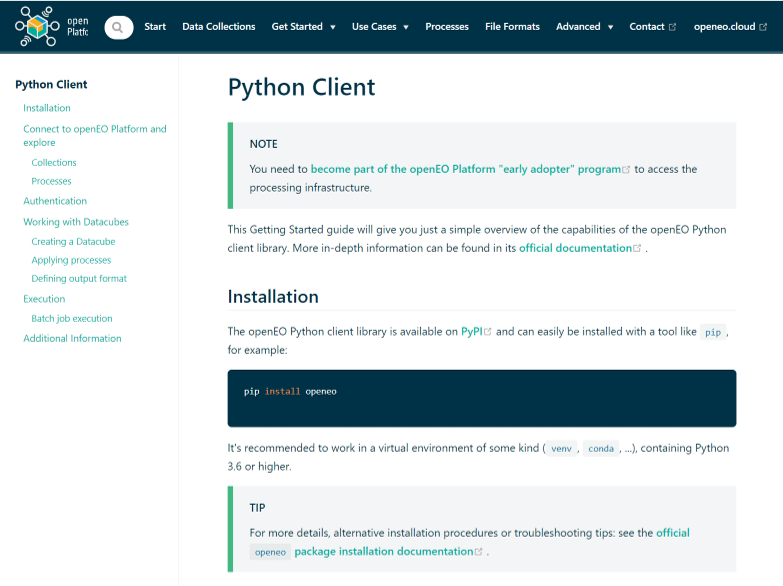

Installation
pip install openeo


					import openeo

					print(openeo.client_version())
Loading a collection
						connection = openeo.connect("https://openeo.cloud")

						  .authenticate_oidc()


						s2_cube = connection.load_collection("SENTINEL2_L2A",

							  spatial_extent={"west":5.1,"east":5.2,"south":51.1,"north":51.2},

							  temporal_extent=["2020-05-01","2020-05-20"],

							  bands=["B03","B04","B08"])
Click here for an overview of all collections.
Click here for the method description of load_collection.
connection.list_processes()
Job management
Two types of jobs: synchronous and batch jobs.Synchronous jobs: fast calculations over small areas, direct download
Batch jobs: heavier operations over larger areas / large time periods, downloaded later using a job ID
Synchronous vs batch jobs
s2_cube.max_time().download("out.geotiff",format="Gtiff")
Batch jobs
								job = s2_cube.execute_batch("out.geotiff",format="Gtiff")

								job = s2_cube.send_job("out.geotiff",format="Gtiff")

								job.start_job()


								job.describe_job()

								job.stop_job()

								job.status()

								job.logs()
Filtering theory
Filtering in practice
s2_cube.filter_temporal(extent="2016-01-01","2016-03-10"])Band filter
s2_cube.band("B02")Spatial filter
s2_cube.filter_bbox(west=5.15,east=5.16,south=51.14, north=51.16, crs=4326)
Band math
Saving bands in a variable
						B04 = s2_cube.band("B04")

						B08 = s2_cube.band("B08")
Doing some band math
ndvi_cube = (B08 – B04) / (B08 + B04)
Index calculation
indices = compute_indices(s2_cube, ["NDVI", "NDMI", "NDGI", "NDRE5"])
Three methods:
						compute_index()

						compute_indices()

						compute_and_rescale_indices()
Click here for an overview of index calculation methods.
Click here for an overview of supported indices.
Applying operations

One-liners
							s2_cube.apply("absolute")

							s2_cube.apply(lambda x: x*2+3)

							s2_cube.apply(lambda x: x.absolute().cos())
See slide on UDFs for difference between apply, apply_dimension, reduce_dimension and apply_neighbourhood
More complex operations
								s2_cube.reduce_dimension(max, dimension="t")


								from openeo.processes import array_element

								def callback(data):

									  band1 = array_element(data, index=0)

									  band2 = array_element(data, index=1)

									  return band1 + 1.2 * band2

								s2_cube.reduce_dimension(callback, dimension="bands")


								def callback2(data):

									  return data.mean()

								s2_cube.reduce_dimension(callback2, dimension="t")
Table of contents
- Introduction
- Field delineation: choosing a model
- History of edge detection
- U-Net
- Pre- and postprocessing
- Field delineation: choosing a platform
- Introduction to openEO
- openEO workflows
- openEO in practice
- Let's start coding: demo notebooks
Questions ?
Contact us on our forum or send us an emailjeroen.dries@vito.be
bart.driessen@vito.be
Reference list
Basavarajaiah, M. (2019). 6 basic things to know about convolution. Medium. Available at: https://medium.com/@bdhuma/6-basic-things-to-know-about-convolution-daef5e1bc411 [Accessed at 17-06-2022]
Ciresan, D., Giusti, A., Gambardella, L., & Schmidhuber, J. (2012). Deep neural networks segment neuronal membranes in electron microscopy images. Advances in neural information processing systems, 25.
Dove, E. S., Joly, Y., Tassé, A. M., & Knoppers, B. M. (2015). Genomic cloud computing: legal and ethical points to consider. European Journal of Human Genetics, 23(10), 1271-1278.
Garcia-Pedrero, A., Gonzalo-Martin, C., & Lillo-Saavedra, M. (2017). A machine learning approach for agricultural parcel delineation through agglomerative segmentation. International journal of remote sensing, 38(7), 1809-1819.
LeCun, Y., Haffner, P., Bottou, L., & Bengio, Y. (1999). Object recognition with gradient-based learning. In Shape, contour and grouping in computer vision (pp. 319-345). Springer, Berlin, Heidelberg.
openEO (2022). openEO Platform. Available at: https://openeo.cloud/ [Accessed at 17-06-2022]
Papers with code (2022). Max Pooling. Available at: https://paperswithcode.com/method/max-pooling [Accessed at 17-06-2022]
Ronneberger, O., Fischer, P., & Brox, T. (2015). U-net: Convolutional networks for biomedical image segmentation. In International Conference on Medical image computing and computer-assisted intervention (pp. 234-241). Springer, Cham.
Szegedy, C., Vanhoucke, V., Ioffe, S., Shlens, J., & Wojna, Z. (2016). Rethinking the inception architecture for computer vision. In Proceedings of the IEEE conference on computer vision and pattern recognition (pp. 2818-2826).
Van der Walt, S., Schönberger, J. L., Nunez-Iglesias, J., Boulogne, F., Warner, J. D., Yager, N., … Yu, T. (2014). Module: future.graph. scikit-image: image processing in Python. PeerJ, 2, p.e453.
Wilson, J. (2019). How instance segmentation works. AI-pool. Available at: https://ai-pool.com/d/could-you-explain-me-how-instance-segmentation-works [Accessed at 17-06-2022]
Zhang, A., Lipton, Z. C., Li, M., & Smola, A. J. (2021). Transposed Convolution. In Dive into deep learning. 13.10.