Developing Applications using Terrascope Platform
Table of Contents
- Virtual Environments
- Accessing Terrascope Notebooks
- Warm-up Exercise
- Interactive Exercise on Phenology Use Case
Virtual Environments
Terrascope provides two virtual environments with necessary tools and data so that you can start coding immediately.
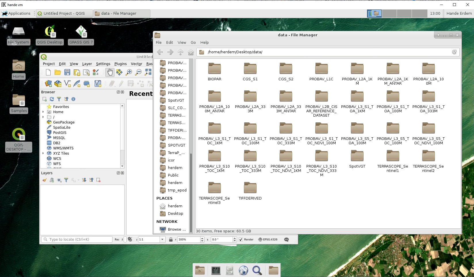
Virtual Machines
Allows developers or scientists to
- access to the available data archives
- use powerful tool set and libraries for further data exploration and analysis (using e.g. the SNAP toolbox, GRASS GIS, and QGIS)
- develop-debug-test applications (in e.g. R, Python or Java)
Jupyter Notebooks
A Notebook is a web application that allows you to create and share scripts that contain live code, equations, visualizations, and narrative supporting text. It is basically a script broken down into several major blocks (cells) that can be executed sequentially. Together with the supporting text cells, the script should be rather easy to comprehend.
The Terrascope Notebooks are based on the Open Source Jupyter notebooks application and tailored to the needs of remote sensing users. Each notebook has direct access to the Terrascope datasets. A notebook facilitates a better and faster understanding of your algorithm by other users.
In this training, we will focus on the Notebooks.
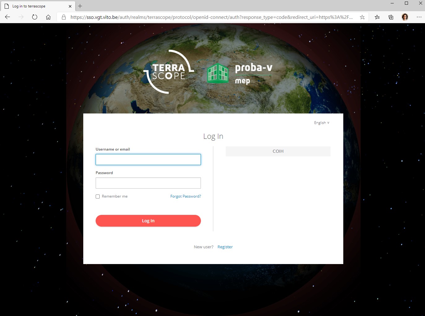
Accessing Terrascope Notebooks
In order to access the Terrascope Notebooks, go to https://notebooks.terrascope.be/ address.You can login if you have an existing account or register if you're a new user.
Terrascope Notebooks
Once you login, you will land on the home page:
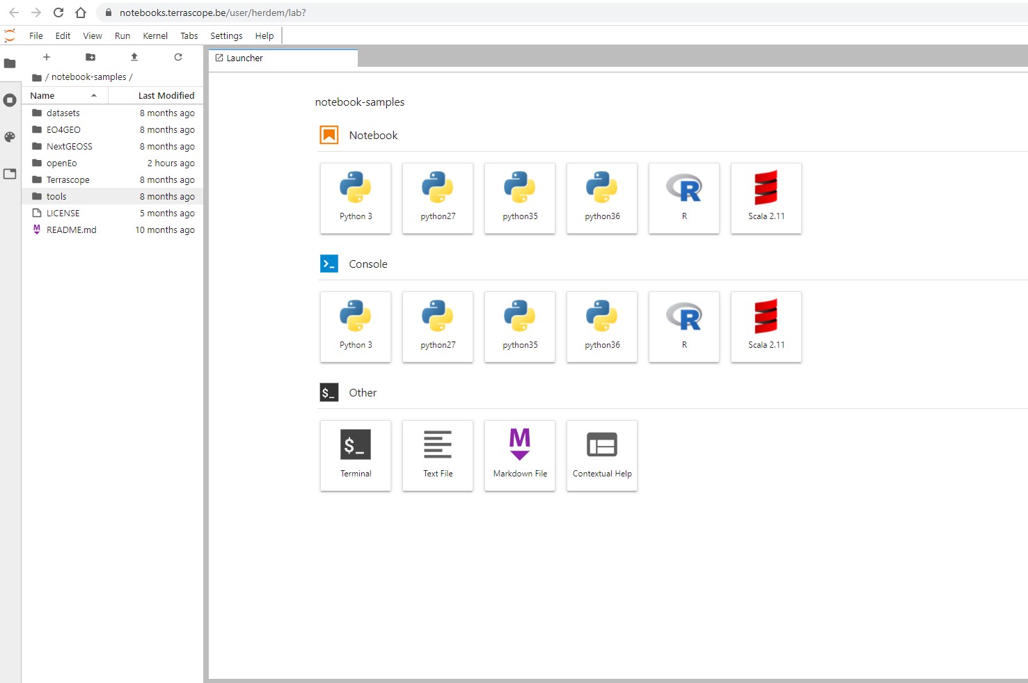
You can either create new notebooks or browse existing ones.
Warm Up
Let's start with a warm up exercise first and do a step-by-step simple band calculation on Sentinel-2 imagery using openEO API.
We'll use OpenEO because it reduces the complexity of handling large amounts and variety of EO data by implementing a standard, with a focus on large scale processing and time series analysis. You can find more information at openeo.org
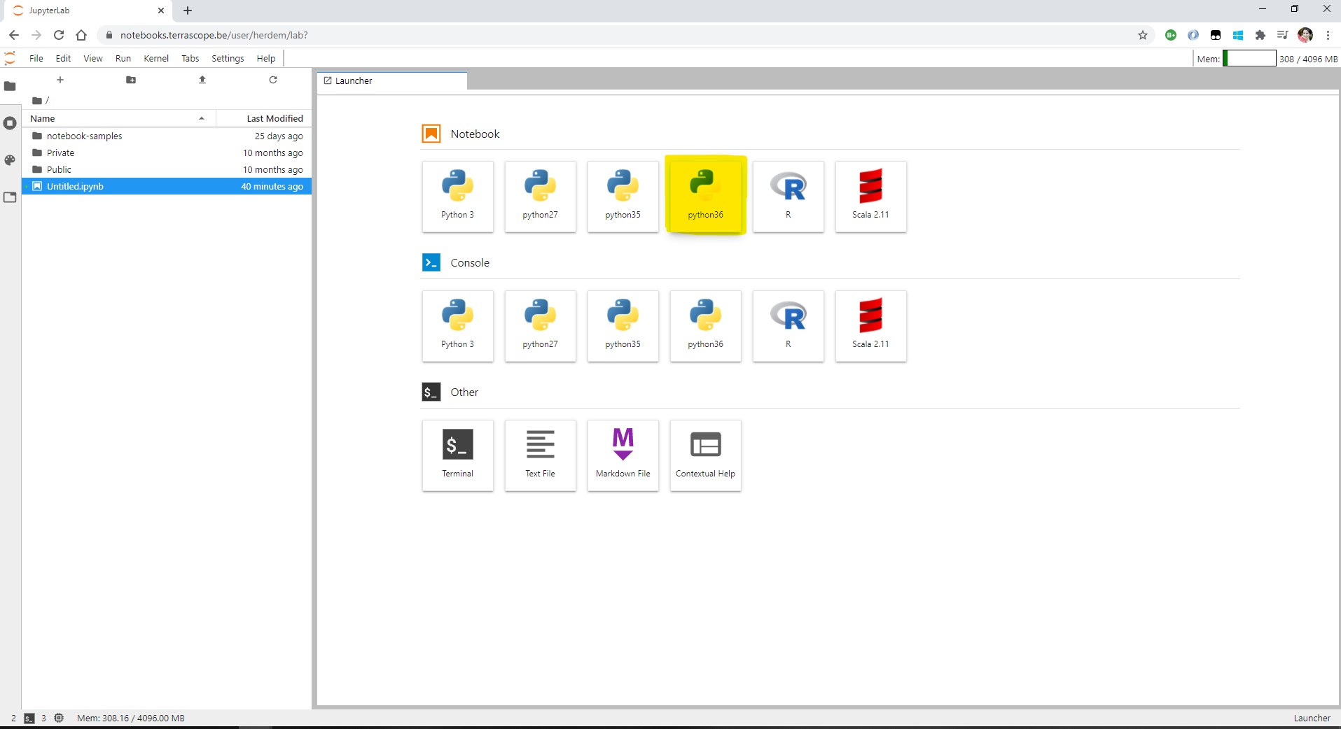
Warm Up
As a first step, go to your Terrascope Notebook homepage and select "python36" notebook to create a new notebook.
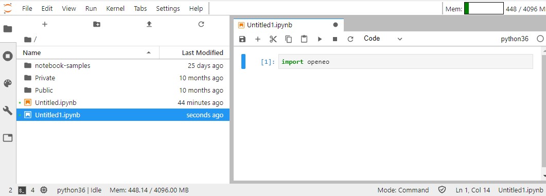
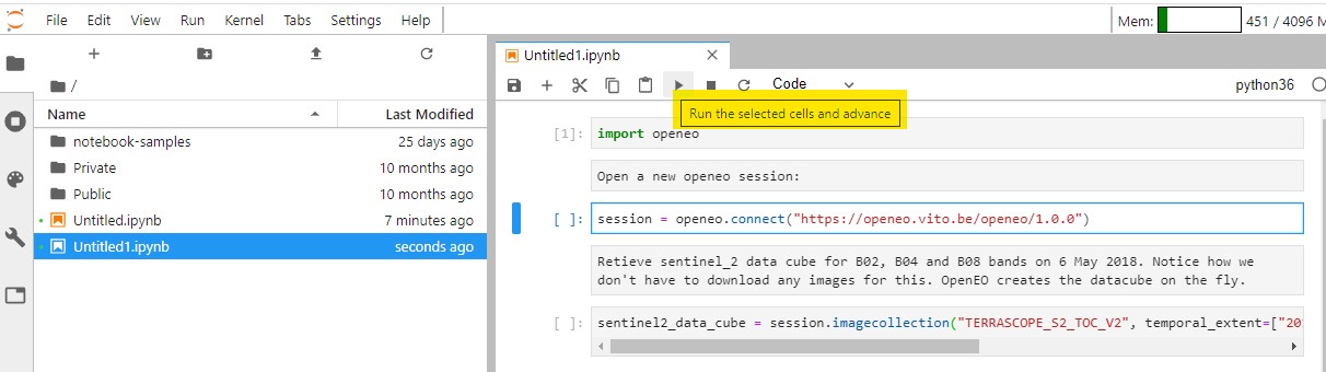
As we are going to use the python client API for openEO, you must start by importing the necessary library. Click on the "+" icon to add a new cell. It will be added automatically as a "Code" cell.
import openeo
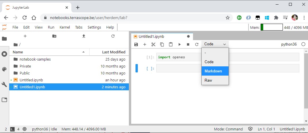
You can also add "Text" cells. These are useful for adding information but won't be executed by the kernel.
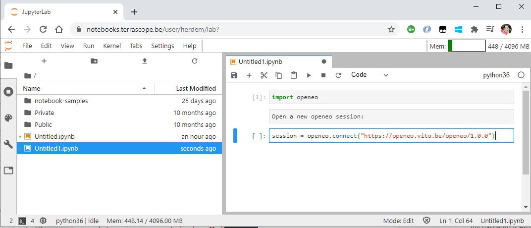
In the next step, we are going to create a new session by connecting to the openEO backend:
session = openeo.connect("https://openeo.vito.be/openeo/1.0.0")
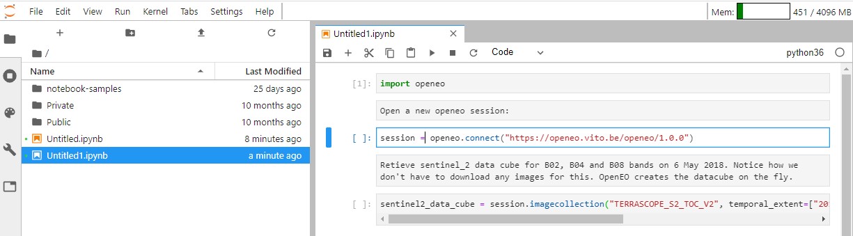
Now that we have the session, we can ask openEO to return us a raster data cube of Sentinel-2 images for 6 May 2018.
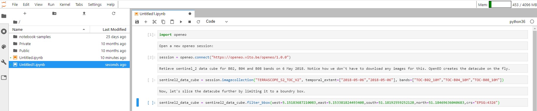
sentinel2_data_cube = session.imagecollection("TERRASCOPE_S2_TOC_V2", temporal_extent=["2018-05-06","2018-05-06"], bands=["TOC-B02_10M","TOC-B04_10M","TOC-B08_10M"])
It is recommended to run the cells as you're adding them to make sure that there are no errors. You can do so by clicking on the "⏵" icon.
We can slice the data cube further by limiting it to a boundry box as shown below:
sentinel2_data_cube =
sentinel2_data_cube.filter_bbox(west=5.15183687210083,east=5.153381824493408,
south=51.18192559252128,north=51.18469636040683,crs="EPSG:4326")
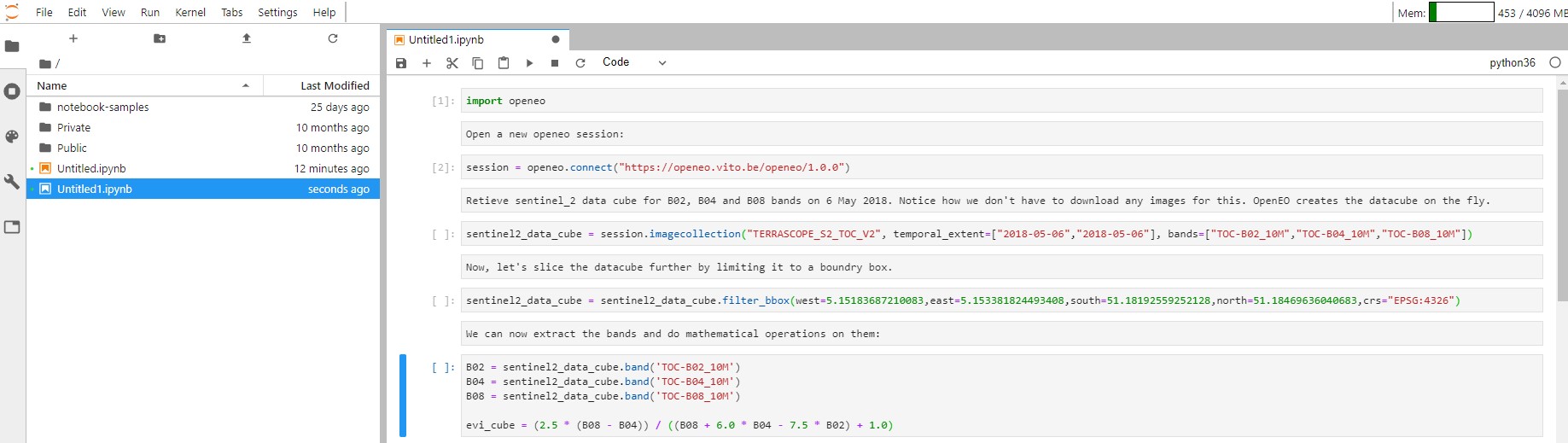
You can extract the bands by calling "band" operation on the openEO data cube on which you can do arithmetic operations. Below, we are calculating the enhanced vegetation index:
B02 = sentinel2_data_cube.band('TOC-B02_10M')
B04 = sentinel2_data_cube.band('TOC-B04_10M')
B08 = sentinel2_data_cube.band('TOC-B08_10M')
evi_cube = (2.5 * (B08 - B04)) / ((B08 + 6.0 * B04 - 7.5 * B02) + 1.0)
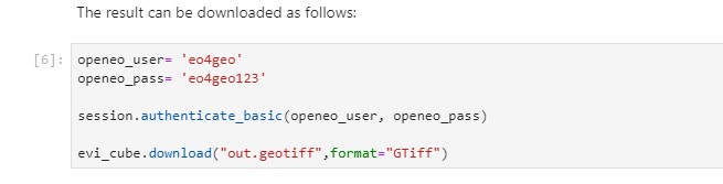
The result can be downloaded after authenticating:
openeo_user= 'eo4geo'
openeo_pass= 'eo4geo123'
session.authenticate_basic(openeo_user, openeo_pass)
evi_cube.download("out.geotiff",format="GTiff")
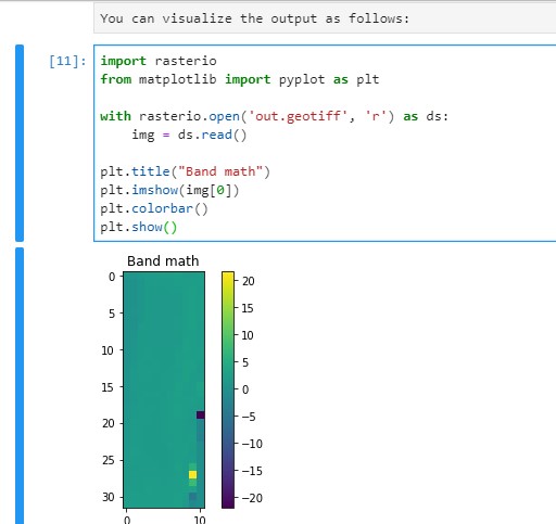
You can visualize the output by using rasterio and matplotlib libraries:
import rasterio
from matplotlib import pyplot as plt
with rasterio.open('out.geotiff', 'r') as ds:
img = ds.read()
plt.title("Band math")
plt.imshow(img[0])
plt.colorbar()
plt.show()
Interactive Exercise on Phenology Use Case
Introduction
Phenology is an important supporting parameter of vegetation that can be derived from remote sensing data. It allows us to evaluate crop conditions, vegetation/crop type in agriculture, and is an indicator for climate change.
Phenology is defined by:
- Start of season, a date and the corresponding value of the biophysical indicator
- End of season, a date and the corresponding value of the biophysical indicator.
Interactive Exercise on Phenology Use Case
Introduction
Deriving phenology accurately requires a sufficiently dense vegetation index time series for a
given pixel or area. At the same time, a sufficiently high spatial resolution is needed, to avoid
noise from sampling heterogeneous areas in a pixel or area. For time series analysis, high spatial
accuracy is also an important requirement.
Today, no single sensor can really satisfy all these
requirements, limiting the accuracy of the predicted phenology parameters. In this use case, we will
use openEO's capability to easily merge multiple datasets with different resolutions:
- Proba-V 10-daily composites: low spatial resolution (300m), but
high temporal resolution
- Sentinel-2: high spatial resolution (10m), low temporal resolution
- Sentinel-1 Gamma0: high spatial & temporal resolution, but no
direct link to phenological
parameters
Interactive Exercise on Phenology Use Case
Introduction
This study will demonstrate the multi sensor data fusion approach by merging three datasets into a single dense vegetation index time series. This is provided as input to a phenology algorithm, which was implemented as a User-Defined Function (UDF), so that it can be easily replaced with other implementations.
Interactive Exercise on Phenology Use Case
Algorithm Overview
Below is a step-by-step overview of the workflow, together with the most important openEO processes that were used to implement them.- Pre-processing Sentinel-2 data
- Load scene classification (load_collection)
- Load- bands 8 and 4 (load_collection)
- Mask NDVI (mask)
- Transform scene classification to binary mask (reduce_dimension)
- Dilate cloud mask (apply_kernel)
- Compute NDVI (ndvi)
- Merging Sentinel-1 Gamma0: (load_collection/resample_cube_spatial/merge)
- Preprocessing and merging PROBA-V 10-daily composites to Sentinel-2 resolution(load_collection/resample_cube_spatial/mask_polygon/merge)
- Apply Deep learning model (GAN) to generate single NDVI (apply_neighborhood/run_udf)
- Pixel wise smooth the resulting time series using Savitzky–Golay filter
- Pixel wise derivation of phenological parameters (apply_dimension/run_udf)
Interactive Exercise on Phenology Use Case
Phenology Jupyter Notebook
- Login to your Terrascope Notebooks account
- Navigate to notebook-samples/openEo/ folder and open data_fusion.ipynb file
- Study and execute the following exercise step by step
- Do not forget to enter the credentials (eo4geo/eo4geo123) in cell #4 of the notebook