Remote Sensing &
Image ProcessingExercise course [UE] - 655.352
Assoc-Prof Dr Stefan LANG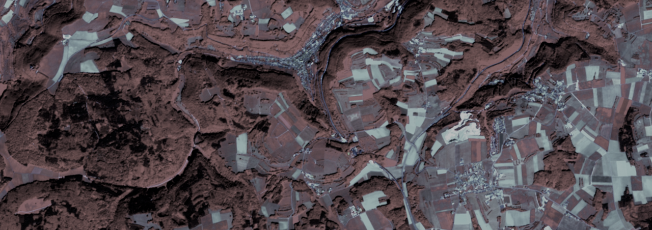

Welcome to this course!
Disclaimer
This is an introductory exercise course to remote sensing. The course material has been developed using tools, concepts and guidelines under the framework of the EO4GEO project. Unless stated otherwise, all rights for figures and additional material are with the author(s).
(c) Z_GIS (S Lang) | 2020
You can navigate through vertical slides by pressing the Down / Up keys on your keyboard or the navigation arrows at the bottom of each slide.
Table of content (ToC)
| 1 | Organisation and introduction |  |
| 2 | Image repositories and data access |  |
| 3 | Specifics of image data |  |
| 4 | Visualising and exploring image data |  |
| 5 | Spatial referencing |  |
| 6 | Radiometric correction |  |
| 7 | Image pre-processing |  |
| 8 | Image classification |  |
| 9 | Validation (accuracy assessment) |  |
| 10 | Publishing results |  |
01 | Organisation and introduction
| Lesson-# | Content | # of topics |
| 01.1 | Course overview and syllabus | 7 |
| 01.2 | Earth observation in practice | 6 |
02 | Image repositories and catalogues
| Lesson-# | Content | # of topics |
| 02.1 | Space and ground infrastructure | 6 |
| 02.2 | Data access | 6 |
03 | Specifics of image data
| Lesson-# | Content | # of topics |
| 03.1 | Image data model | 7 |
| 03.2 | Histograms | 3 |
04 | Visualising and exploring image data
| Lesson-# | Content | # of topics |
| 04.1 | Sensors and metadata | 2 |
| 04.2 | Image handling | 3 |
| 04.3 | Band combination | 3 |
05 | Spatial referencing
| Lesson-# | Content | # of topics |
| 05.1 | Spatial vs. geometric correction | 6 |
| 05.2 | GCP collection and referencing | 5 |
06 | Radiometric correction
| Lesson-# | Content | # of topics |
| 06.1 | Radiometric measurement | 3 |
| 06.2 | Atmospheric correction | 2 |
| 06.3 | Topographic correction | 3 |
07 | Image pre-processing
| Lesson-# | Content | # of topics |
| 07.1 | Band maths | 3 |
| 07.2 | Filtering | 5 |
| 07.3 | Image fusion and PCA | 3 |
08 | Image classification
| Lesson-# | Content | Topics |
| 08.1 | Multi-spectral classification | 5 |
| 08.2 | Supervised classification | 5 |
09 | Validation (accuracy assessment)
| Lesson-# | Content | Topics |
| 09.1 | Ground reference and error matrix | 4 |
| 09.2 | Product validation | 3 |
10 | Publishing results
| Lesson-# | Content | Topics |
| 10.1 | tbd | x |
| 10.2 | tbd | x |
01 | Organisation and introduction
Remote Sensing & Image Processing
01.1 | Course overview and structure
Learning objectives [lesson 1.1]
Understand the structure and content of the course, as well as its requiements and objectives
- Get an overview of the software environment and datasets being used
01.1 | Course overview and structure
Content and topics [lesson 1.1]
| # | Content |
| i | Overview course structure and learning objectives |
| ii | Experience and prior knowledge |
| iii | Road map and syllabus |
| iv | Workload, assignments and grading |
| v | Literature and reference material |
| vi | Software and data being used |
| vii | Tutorials |
01.1 (i) Course structure and learning objectives
The course is structured in the following way:
Units
Lessons
Topics
Learning objectives are specified on the level of lessons, meaning there is one learning objective (or more related ones) provided for each lesson.
Altogether, there are 10 units with 2-4 lessons each. Around one-hundred topics are covered by this course. Each topic is linked, when applicable, with a concept from the EO4GEO Body of Knowledge (BoK) of the EO*GI sector in the following form:
| # | Content | BoK concept |
| Topic number | Topic | Permalink to BoK |
01.1 (ii) Experience and prior knowledge
The course relies on general interest and prior knowledge in remote sensing. While not a formal prerequisite, it is recommended to having completed or being enrolled in parallel to the introductory lecture course “Remote Sensing and Image Processing” (VL 655.351).
This course conveys specific technical skills. If you want to familiarize even better with the software environment, you may enroll to "Introduction to GIS" (UE 655.332).
General skills are acquired according to Bloom's taxonomy of skills levels (see below, @Assignments).
01.1 (iii) Course schedule and syllabus
Time and place
This course takes place Wednesdays, 16.00 - 18.00 in the GI Lab. Press "show schedule" for more details on the current syllabus and schedule for this semester. Updates or any occuring changes you may find in PlusOnline.

Depending on the Covid-19 regulations, the course is offered in hybrid or online mode.
01.1 (iv) Workload, assignments and grading
Workload
UE = "continuous assessment course". What does that mean? The course implies mandatory presence, active participation, and submission of all assignments; on the other hand, no final examination takes place!
The course consists of 7-8 present dates with 30 min theoretical background and revision assignments; 60 min joint practical exercise including discussion of relevant concepts. Tutorials are offered 2-3 times per semester.
2 ECTS credits = 50 h student workload (~ 1/3 course, 2/3 homework)
01.1 (iv cont.) Workload, assignments and grading
Assignments (A1 … A5)
- Assignments will be announced in the respective class
- ... need to be delivered in time to receive feedback (watch your calendar in BlackBoard)
- ... one attempt at a time
Please obey the following naming convention:
A[n]_[lastname], e.g. A1_Johnson. Please
use PFD format exclusively!
Grading: < 50% = insufficient |...| > 85% = very good. Grade distribution:
| Assignment | Points |
| 1 | 10 |
| 2 | 15 |
| 3 | 15 |
| 4 | 15 |
| 5 | 20 |
01.1 (iv cont.) Workload, assignments and grading
Assignments (A1 … A5)
Assignments and the respective learning outcomes follow the Bloom's taxonomy of skills levels (Anderson 2001). That means skills acquired in the assignments range from basic (remember) in the earlier, to advanced (create) in the later, assignments.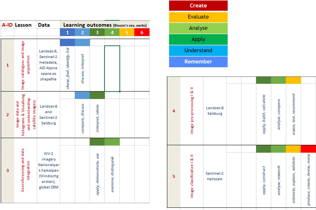
01.1 (v) Literature and reference material
Selected text books are available in the joint library (Material Science building, Booth #32)

Please see the following table of recommended books!
01.1 (vi) Software and data sets used
- Satellite data
- All data are located in the MyFiles share (see Blackboard)
- Data are real data, no ‘fake’ or fabricated data
- NB: data may be subject to license agreements restricting their usage to research or educational purposes. Copying or using those data for any other purpose is prohibit.
- Software: ArcGIS Pro by ESRI (Image Analysis components)
- It is easy to use, convenient look & feel
- Workflows are pre-defined and guided (‚one-click‘)
- You can stay within one environment (no change of software, transfer of data, etc.)
- But: ArcGIS Pro is a commercial software package

01.1 (vii) Tutorial
Tutor: Christina Zorenböhmer
Email: christina.zorenboehmer@sbg.ac.at
Assignments and tutorials will give you the opportunity to get some hands-on experience with the platforms, software, and tools used in remote sensing.
Assignment 1 on image acquisition and online platforms will be handed out next week!
01.2 | Earth observation in practice
Learning objectives [lesson 1.2]
- Get to know the role of remote sensing in Earth observation and Copernicus
- Familiarize with the practical dimension of satellite Earth observation by examples
- Learn the principle of the image analysis workflow and image processing chain
- Understand the difference between pixel- and object (or region-) based approach
01.2 | Earth observation in practice
Content and topics [lesson 1.2]
| # | Content | BoK concept |
| i | Satellite remote sensing | Remote Sensing Platforms and Systems |
| ii | What is Copernicus? | Copernicus Programme |
| iii | EO @ Z_GIS | n/a |
| iv | Image processing chain | Image Processing |
| v | Pixel- vs. object-based approach | Object-based image analysis (OBIA) |
01.2 (i) Satellite remote sensing
"From time immemorial people have used vantage points high above the landscape to view the terrain below. From these lookouts they could get a ‘bird’s eye view’ of the region. They could study the landscape and interpret what they saw. The advantage of collecting information about the landscape from a distance was recognized long ago. Remote sensing as we know it today is the technique of collecting information from a distance. By convention, ‘from a distance’ is generally considered to be large relative to what a person can reach out and touch, hundreds of meters, hundreds of kilometers, or more. The data collected from a distance are termed remotely sensed data." (Stan Aronoff, 1989)

01.2 (i cont.) Satellite remote sensing and Earth observation
Earth observation is one out of three main space assets.
- Satellite navigation
- Satellite communication
- Satellite / Earth observation (EO)
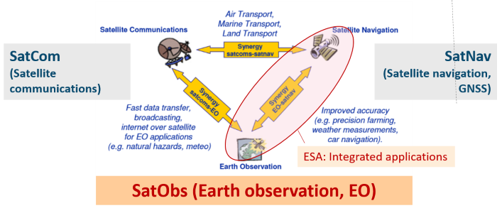
01.2 (1 cont.) Satellite navigation
The European satellite navigation (SatNav) programme is called Galileo. With EGNOS, the European differential global positioning system, it belongs to the world spanning global navigation satellite systems (GNSS).
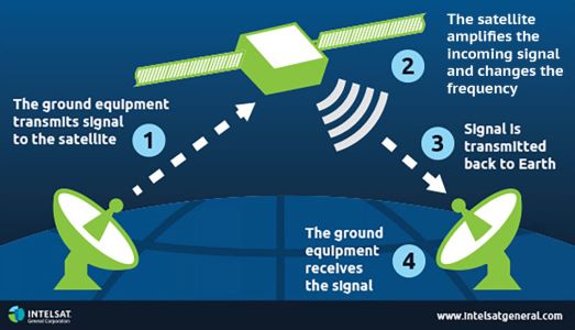
01.2 (1 cont.) Satellite communication
Communication via satellites (SatCom) allows telecommunication all around the globe. Communication satellites receive signals from Earth and retransmit them by a transponder.
01.2 (1 cont.) Earth observation
Earth observation (EO) is the systematic usage of satellite remote sensing technology for continuous or on-demand imaging or measuring of the Earth surface

01.2 (ii) What is Copernicus?
Copernicus is the conjoint Earth observation programme by the European Space Agency (ESA) and the European Commission (EC) as laid out in the European Space Policy.
Copernicus uses satellite technology to support monitoring the state of our environment and our social well-being. Here are some of the main aspects observed by Copernicus (see lesson 2.2):
- the conditions of the atmosphere or our land and marine ecosystems
- the use of the land for forestry and agriculture
- the process of urbanisation
- the likely climate change impacts
- the natural and man-made disasters
- our human security and public health
01.2 (ii cont.) What is Copernicus?
01.2 (ii cont.) Copernicus idea
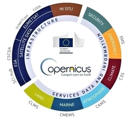
Copernicus comprises three major components.
- Space segment
- Integrated ground segment
- Data access and information services
01.3 (iii) EO @ Z_GIS
...

01.4 (iv) Image processing chain
...
01.5 (v) Pixel- vs. object-based approach
...
02 | Image repositories and data access
Image Processing & Analysis
02.1 | Space and ground infrastructure
Learning objectives [lesson 2.1]
Get an overview of different types of satellite sensors and platforms
Compare two flagship satellite programmes (Landsat vs. Sentinel)
Conceptualise the term big EO data
Understand the principle of data acquisition and retrieval
- Get to know the Copernicus data and information access service (DIAS)
02.1 | Space and ground infrastructure
Content and topics [lesson 2.1]
| # | Content | BoK concept |
| i | Space segment - Earth observation satellites | Platforms and sensors |
| ii | Examples: NASA Landsat & Copernicus Sentinel | * |
| iii | Big EO data | * |
| iv | Integrated ground segment | Next-generation SDIs |
| v | Data and information access service (DIAS) | * |
| vi | (Semantic) content-based image retrieval | Semantic enrichment |
02.1 (i) Space segment - EO satellites
EO for societal (and environmental) benefit: GEO/SS Many initiatives are in place to promote the peaceful use of EO satellites.
The intergovernmental Group on Earth Observations (GEO) is a strong
driver behind the integration of various kinds of EO systems globally into a system of systems (GEOSS). Copernicus is the European
contribution to GEO.
EO for sustainable development: EO4SDGEO (and GNSS) is crucial in supporting the achievement of the development goals (SDGs) as
recognised by the UN. UNOOSA provides an overview
on the potential of space in supporting the SDGs.

02.1 (i) Space segment - EO satellites
Copernicus is like a stage where different actors with their favourite instruments play together in a band.

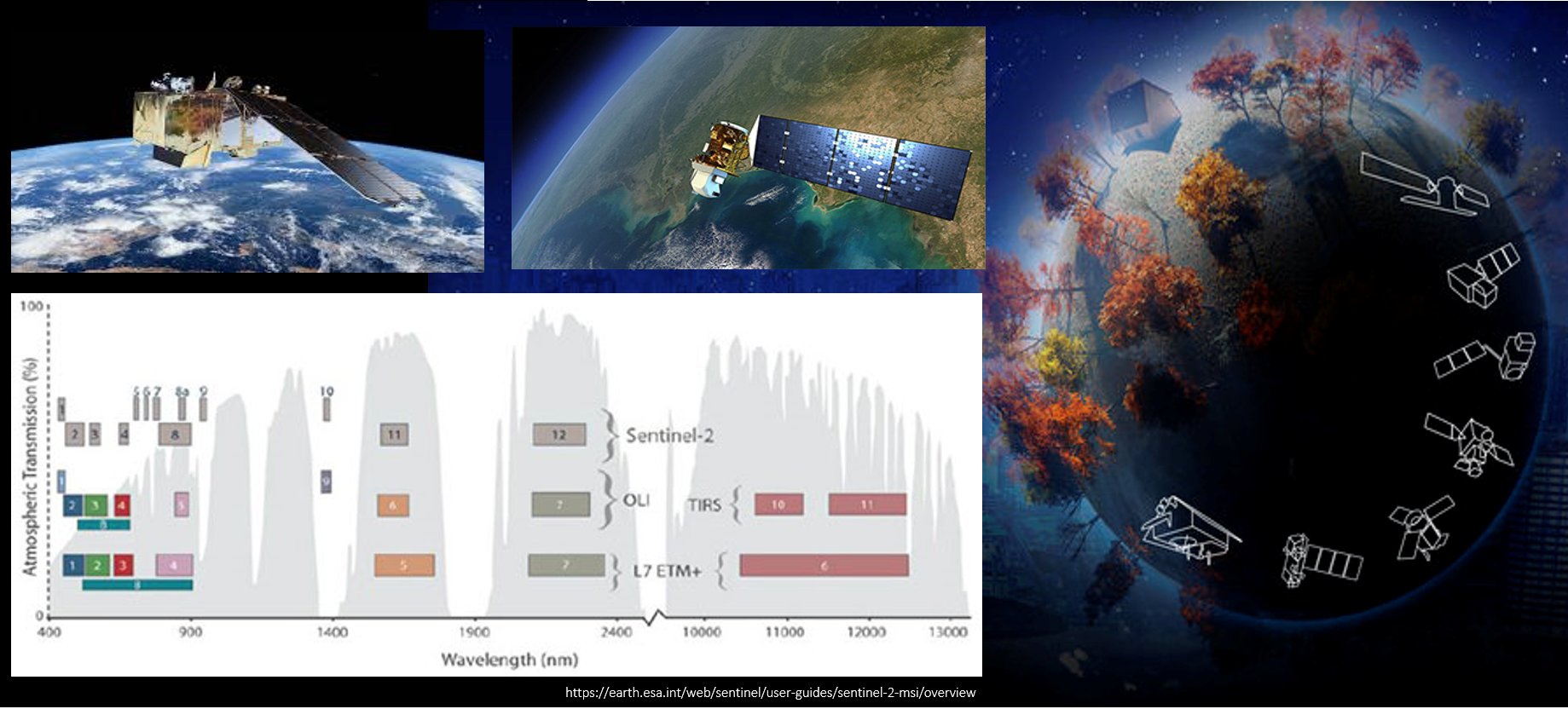
02.1 (ii) Examples: NASA Landsat & Copernicus Sentinel
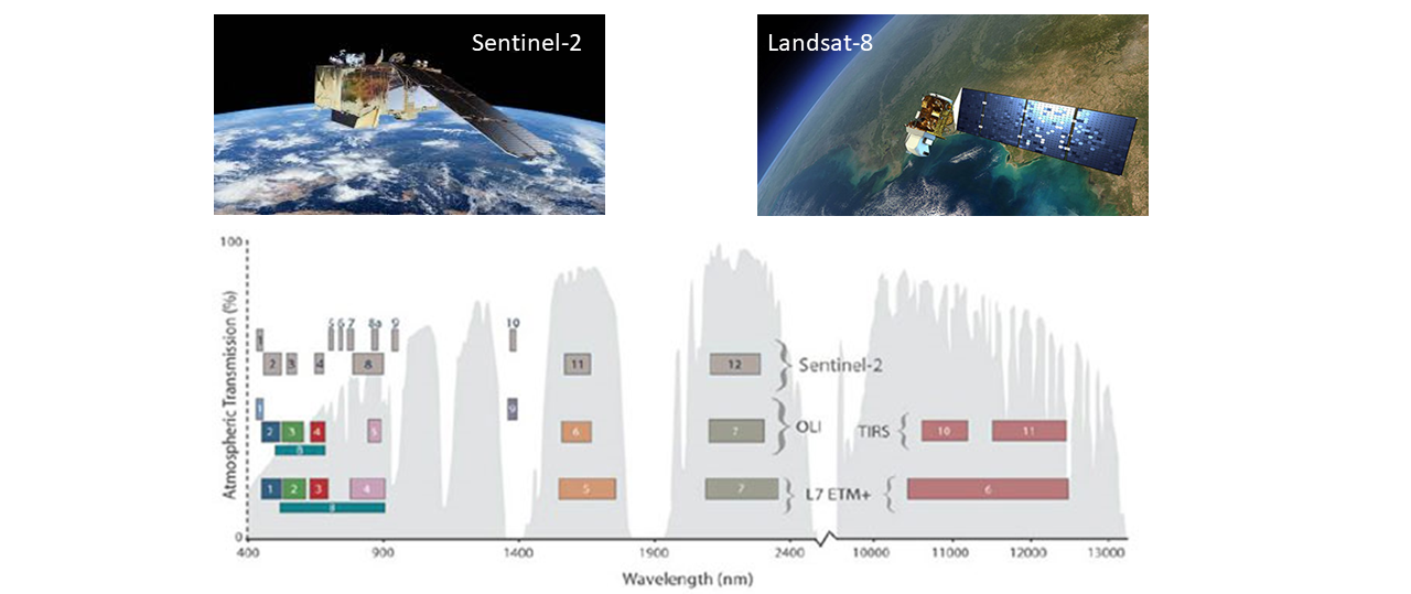
Landsat-8 is the flagship of the long-lasting Landsat programme by NASA and USGS in the United States. The onboard instruments (sensors) of Landsat-8 are called OLI (optical) and TIRS (thermal). The Sentinel family is the backbone of the Copernicus EO space asset with Sentinel-2 carrying the optical instrument MSI.
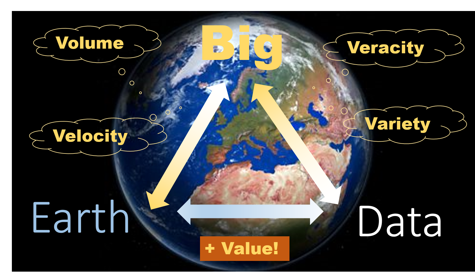
02.1 (iii) Big EO data
The 4 "Vs" (volume, velocity, veracity, variety) usually describe the big data paradigm. A 5th V ('value') in EO asummes the investment in Space infrastructure stimulates an emerging market in the downstream sector.
02.1 (iii cont.) Big EO data
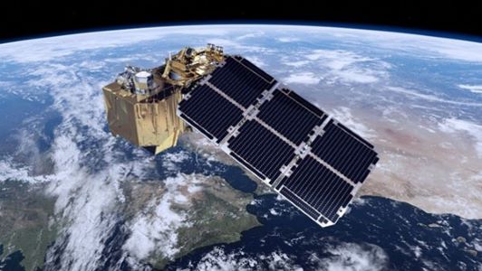
The Copernicus space infrastructure programme is mainly represented by a suite of satellites called the 'Sentinels'.

02.1 (iv) Integrated ground segment
The Copernicus integrated ground segment (IGS) includes
- Receiving stations
- Satellite data storage systems
- Information access services
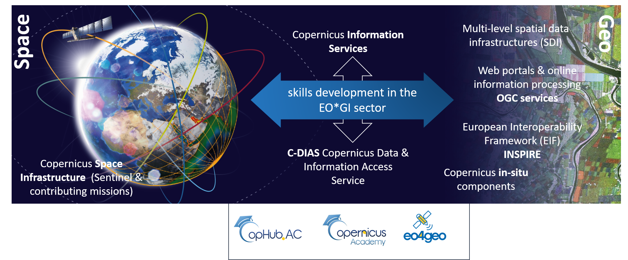
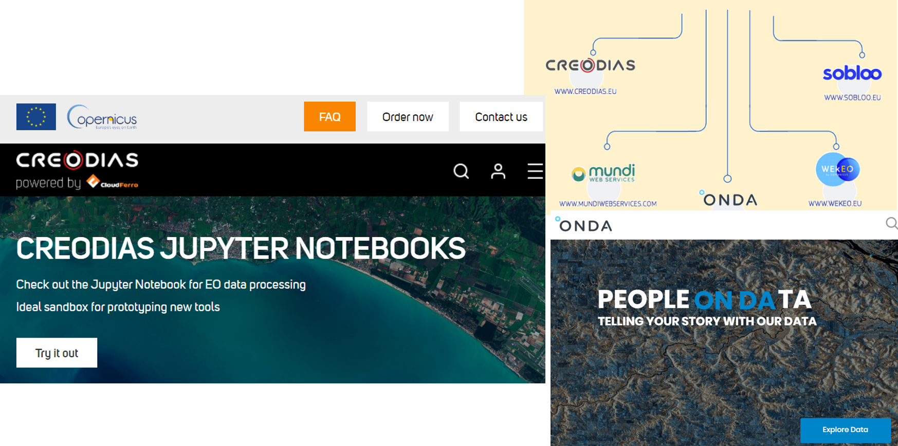
02.1 (v) Data and information access service (DIAS)
02.1 (vi) (Semantic) content-based image retrieval
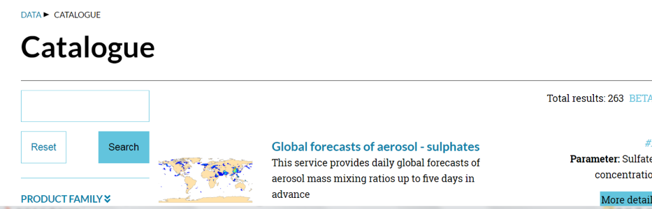
How to find suitable imagery in a data catalogue (see lesson 2.2)? Consider the following scenario.
A public authority needs to report on water quality of large swimming lakes (could be in Austria, Switzerland, northern
Italy, southern Germany, etc.) during high season over the past three years. For this purpose a service provider (EO company)
is contracted to deliver value-adding information products based on satellite images. The EO expert in the company needs to
search for a suitable set of images. (More Copernicus use cases you can find here.)
The expert may consider the following search criteria: (1) time window, (2) geographical focus (AOI), (3) cloud cover, (4) thematic focus,
(5) monitoring period, more specifically:
|
 |
02.2 | Data & information access
Learning objectives [lesson 2.2]
Get to know different sources and options for data search via free platforms
Understand how to search and acquire VHR satellite imagery ('tasking) from commercial data providers
- Learn how to access information layers from Copernicus services
02.2 | Data & information access
Content and topics [lesson 2.2]
| # | Content | BoK concept |
| i | Earth explorer (USGS) | * |
| ii | Sentinel hub and playground | * |
| iii | Commercial VHR data portals | * |
| iv | Google Earth Engine | * |
| v | Proba-V mission exploitation platform | * |
| vi | Copernicus service platforms | * |
02.2 (i) Earth explorer (USGS)


02.2 (ii) Sentinel hub and playground
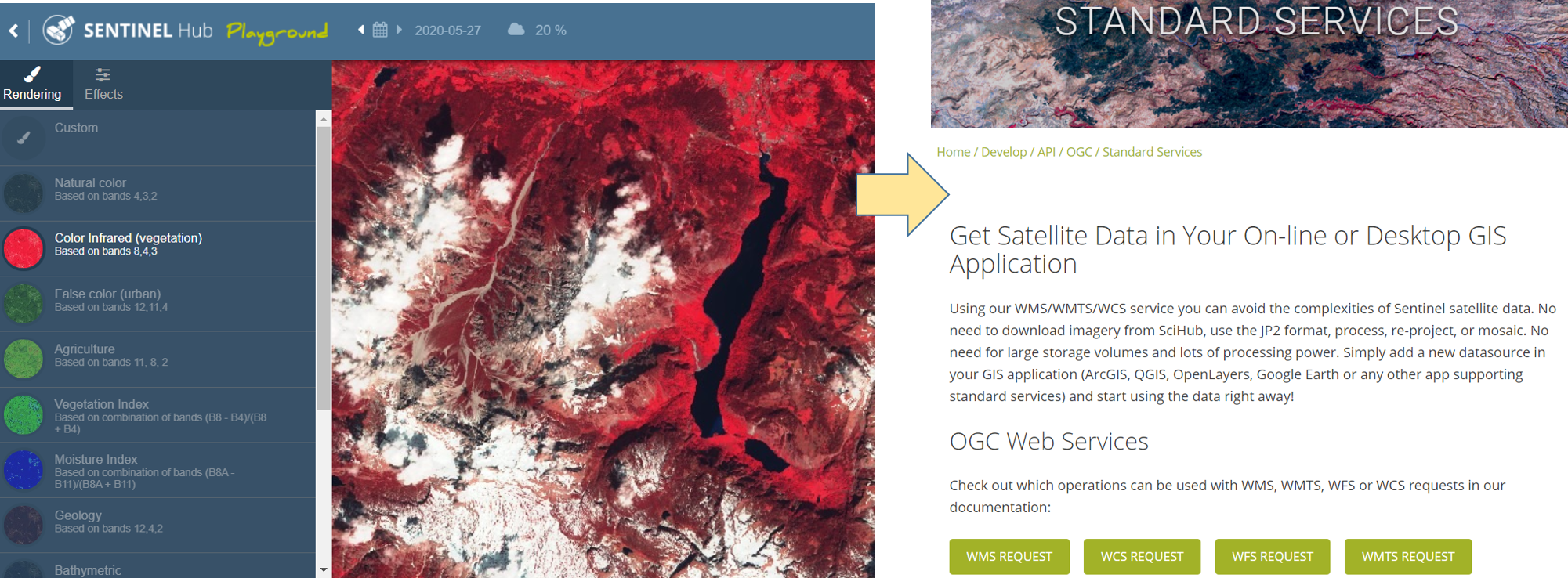
02.2 (ii cont.) Copernicus Open Access Hub

02.2 (iii) Commercial VHR data portals
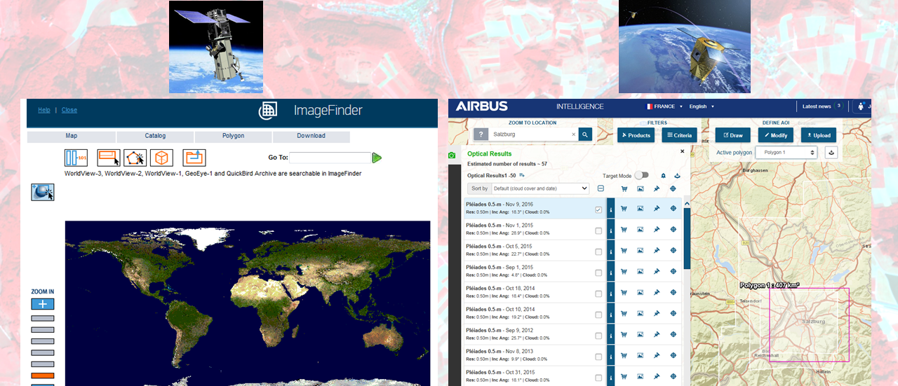


02.2 (iii cont.) Commercial VHR data portals
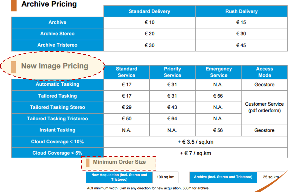
A general note on pricing schemes
Freely available data (Landsat, Sentinel, etc.) involve billions of public investment. Commercial satellites are run by private companies that seek for return of investment.
Cost model factors include:
|
 |
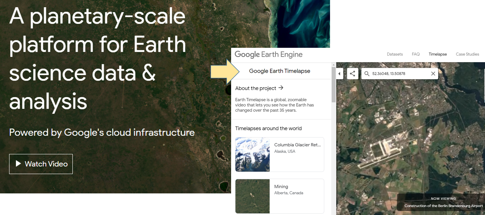
02.2 (iv) Google Earth Engine
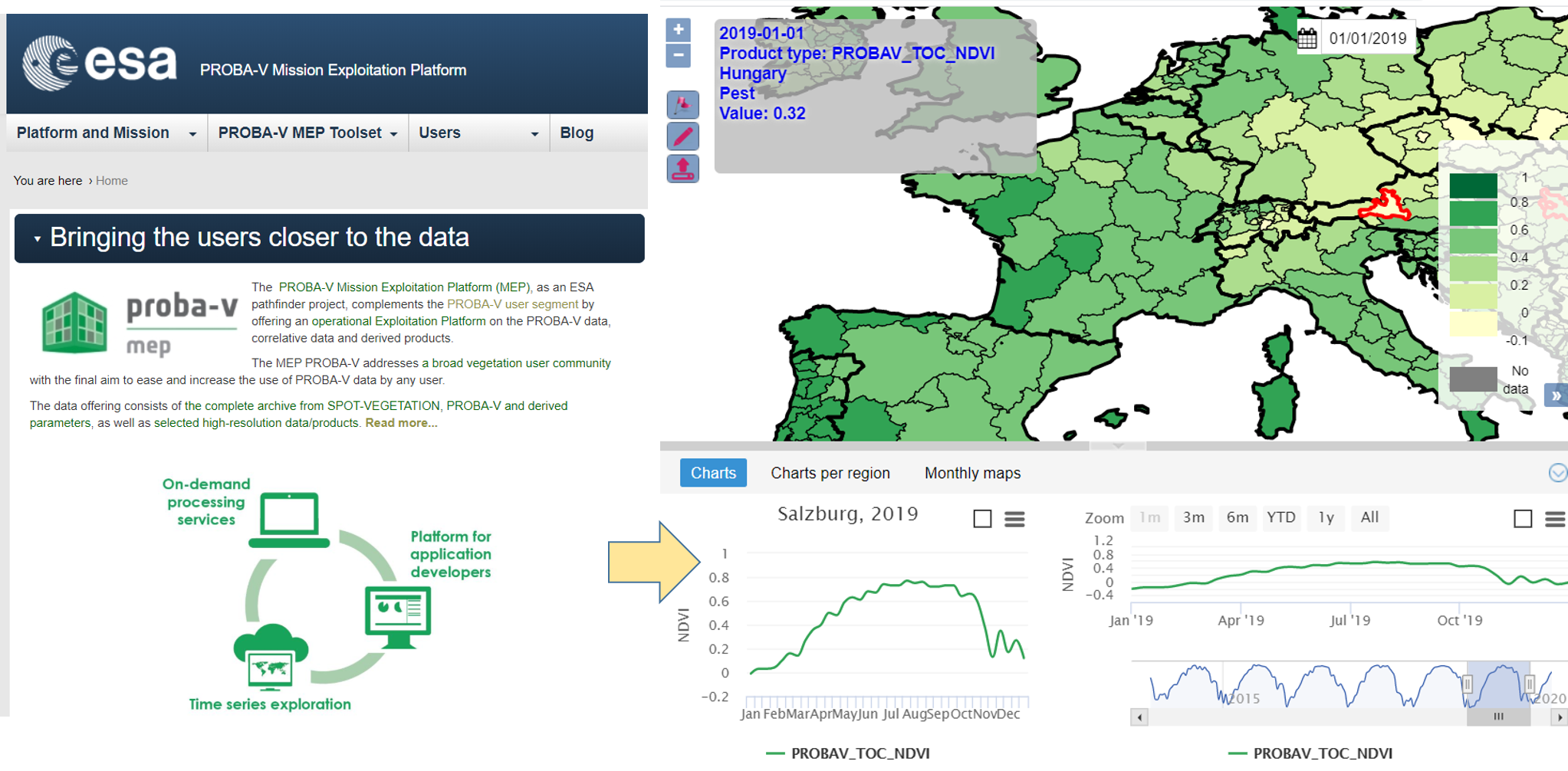
02.2 (v) Proba-V mission exploitation platform
02.2 (vi) Copernicus service platforms
The fundamental objective of Copernicus is to support policies, regulations, conventions, and directives with a defined portfolio geospatial information services in the following areas:
02.2 (v) cont. Copernicus service platforms
Copernicus services
There are six so-called Copernicus [core] services in six major thematic areas.


Land monitoring
The Copernicus Land Monitoring service (CLMS) aims at monitoring the Earth.


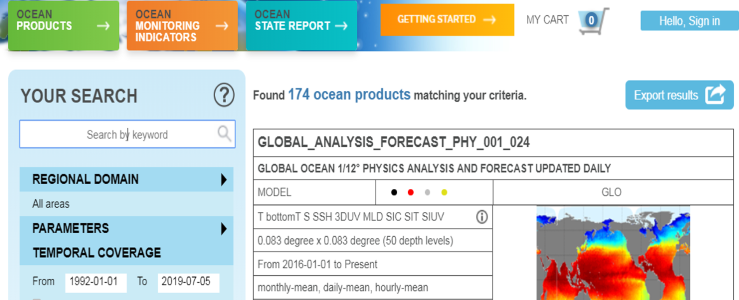
Ocean monitoring
The Copernicus Marine Environment Monitoring service (CMEMS) focuses on the global ocean.

Atmosphere monitoring
The Copernicus Marine Environment Monitoring service (CAMS) focuses on the global ocean.

Climate change
The Copernicus Climate Change service (C3S)


Emergency management
The Copernicus Emergency Management service (CEMS)


Human security
The Copernicus Security service contains of three subservices, (1) Maritime surveillance, (2) Border surveillance and the (3) support to European External Action (SEA)

The Copernicus ecosystem
Copernicus engages different actor groups.
- Data providers
- Service providers
- Users and stakeholders

Data providers
Next to the Sentinel satellites there is a series of contributing missions, including commercial providers of very high (spatial) resolution (VHR) data.

Include the example of Planet and Skysat (completion of constellation such that every location on Earth is visible by 7 satellites)
Service providers
...
Users and stakeholders
...
03 | Specifics of image data
Image Processing & Analysis
03.1 | Image data model
Learning objectives [lesson 3.1]
<<<<<<< HEAD
Understand the specifics of image data as a special case of raster data
Familiarize with top-view characteristics of image data as well as the difference between panchromatic and multispectral images
Learn to distinguish between different resolution types
Learn how to use spectral profiles as an analysis tool
Understand different image storage strategies
Understand the specifics of image data as a special case of raster data
Familiarize with top-view characteristics of image data as well as the difference between panchromatic and multispectral images
Learn to distinguish between different resolution types
Learn how to use spectral profiles as an analysis tool
- Understand different image storage strategies
03.1 | Image data model
Content and topics [lesson 3.1]
| # | Content | BoK concept |
| i | What are image data? | Properties of digital imagery |
| ii | Vector vs. raster data representation | The raster model |
| iii | Resolution types | Spectral resolution |
| iv | Image matrix and image regions | * |
| v | Panchromatic vs. multi-band images, feature space | Radiometric resolution |
| vi | Spectral profiles | * |
| vii | Storage options | Data storage |
03.1 (i) What are image data?
Image data are a specific type of raster data representing a subset of the Earth's surface by recording the continous phenomenon of radiation reflectance. Image data are captured by sensors mounted on different platforms, such as ballons, drones, aircrafts, and satellites.
03.1 (ii) Vector vs. raster data representation
Vector data are used to represent spatial discreta, while raster data are the appropriate data model for spatial continua.

03.1 (iii) Resolution types
There are four different resolution types: spectral, spatial, radiometric, temporal resolution

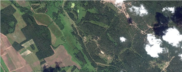
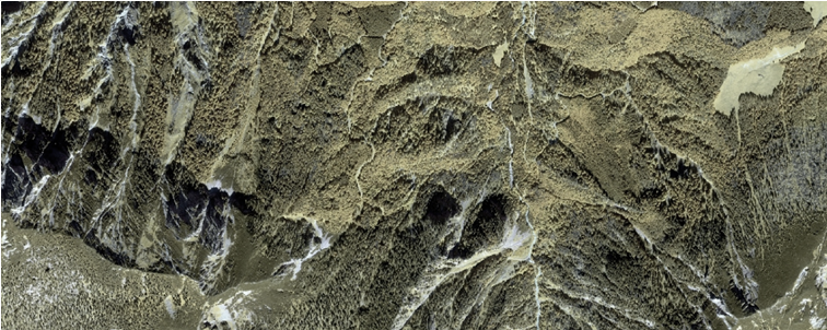
Pléiades image of the city of Salzburg with 0.5m spatial resolution.
03.1 (iv) Image matrix and image regions
An image matrix (or pixel array) is defined by (i) coordinates of origin, (ii) resolution (pixel size), (iii) extent (dimension)

03.1 (v) Panchromatic vs. multi-band images, feature space
Satellite imagery consists of several co-registered pixel arrays representing a combination of different spectral bands.

The visual effect of combining different spectral bands can be interpreted by humans or machines in order to derive semantic information (e.g. land cover classes).
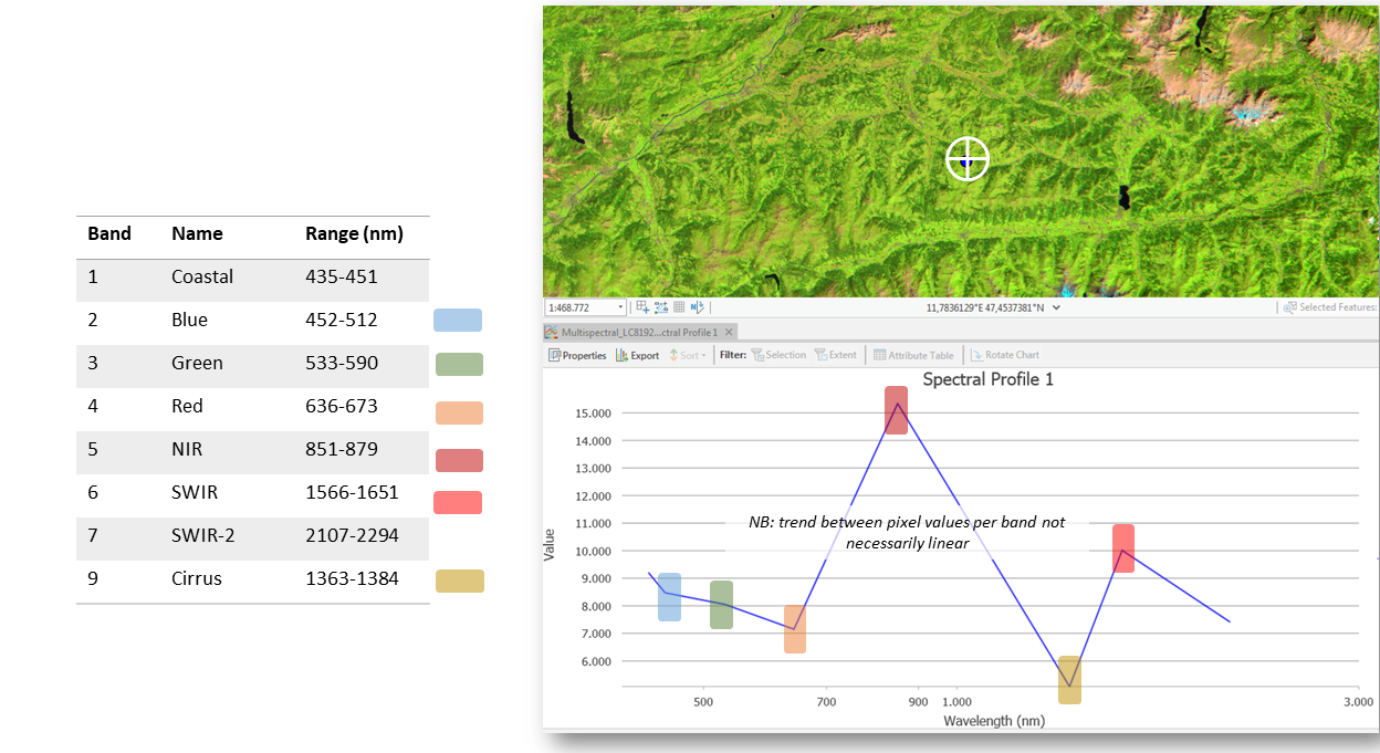
03.1 (vi) Spectral profiles
Spectral profiles help determine the spectral properties of a given pixel (i.e., at a specific location)
03.1 (vii) Storage options
There are different options for storing multi-band images, band-interleaved by line (BIL), band-interleaved by pixel (BIP), and band sequential (BSQ)

03.2 | Histograms
Learning objectives [lesson 3.2]
Understand the frequency distribution of pixels in images
Learn how to generate and to read histograms
03.2 | Histograms
Content and topics [lesson 3.2]
| # | Content | BoK concept |
| i | Value frequency distribution | * |
| ii | Interpretation of histograms | Histograms |
| iii | Histogram generation | * |
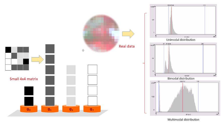
03.2 (i) Value frequency distribution
Histograms
What is a histogram? A histogram is a statistical chart technique providing a compact overview of the data in an image than knowing the exact value of every pixel.

03.2 (ii) Interpretation of histograms
03.2 (iii) Histogram generation
Interactive excercise

Here you find a interactive Jupyter notebook on how to convert a sequence of digital numbers stored in a BIL format into a histogram
04 | Visualising and exploring image data
Image Processing & Analysis
04.1 | Sensors and metadata
Learning objectives [lesson 4.1]
- Learn what typical metadata are produced by satellite imagery
- Understand how metadata of image collections (e.g. Sentinel-2) can be used to better understand the availabilty and quality of satellite data
04.1 | Sensors and metadata
Content and topics [lesson 4.1]
| # | Content | BoK concept |
| i | Sensor characteristics (Landsat/Sentinel-2 vs. Worldview-2) | * |
| ii | Satellite image metadata analysis (webtool EO Compass) | * |
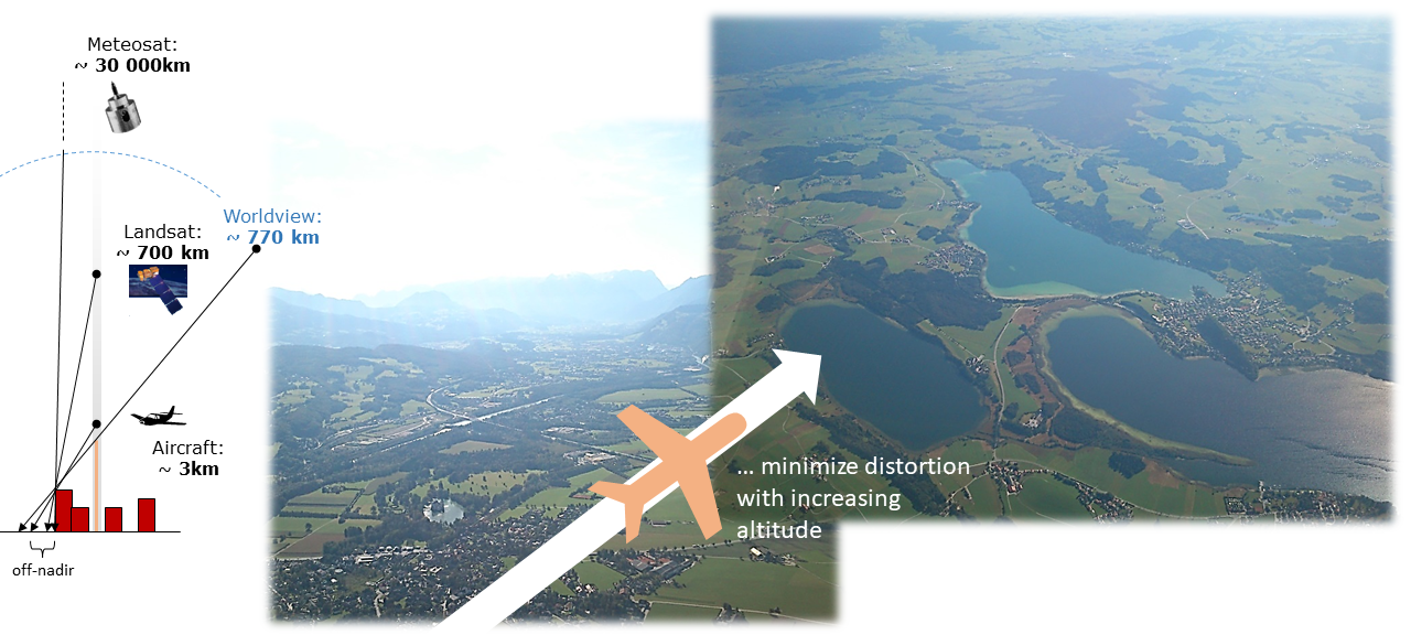
04.1 (i) Sensor characteristics (Landsat/Sentinel-2 vs. Worldview-2)
Typical features of HR vs. VHR sensors
Using the examples of two representatives of the high-resolution (HR) optical satellites family (Landsat-8 & Sentinel-2) and a VHR satellite (Worldview-2)
04.1 (ii) Satellite image metadata analysis
The EO Compass
A stand-alone webtool to understand the global coverage and quality of Sentinel-2 image acquisition based on image metadata analysis.

04.2 | Image handling
Learning objectives [lesson 4.2]
- Practice the handling of image data in dedicated software environment
- Learn how to use the ArcGIS Pro Image Analysis module
04.2 | Image handling
Content and topics [lesson 4.2]
| # | Content | BoK concept |
| i | ArcGIS Pro Image Analysis module | * |
| ii | Organising and loading image data | * |
04.2 i ArcGIS Pro Image Analysis module
Visualising images in ArcGIS Pro

04.2 iii Organising and loading image data
Visualising images in ArcGIS Pro
 Open multi-band image via container file (left). Make background transparent (right).
04.3 | Band combinations
Learning objectives [lesson 4.3]
- Understand how to visualise, manipulate, and interact with, image data
- Learn what general principles apply when interpretating them (including change of band combinations)
04.3 | Band combinations
Content and topics [lesson 4.3]
| # | Content | BoK concept |
| i | Visualising image data | Layer stack |
| ii | Range adjustment and resampling for viewing | Raster resampling |
| iii | Band combinations (incl ArcGIS Pro presets) | Visual interpretation |
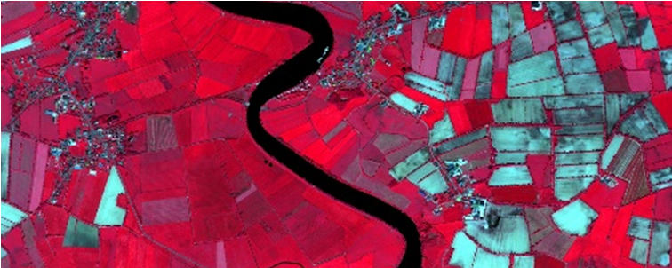
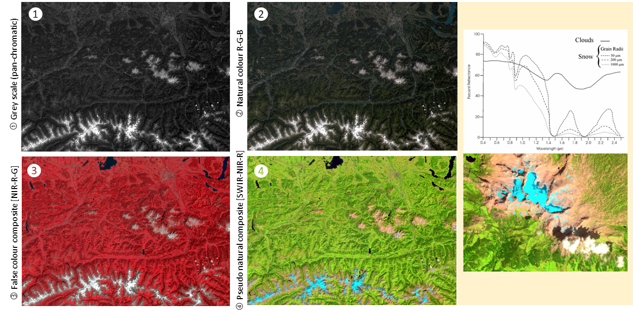
04.3 (i) Visualising image data
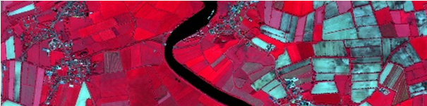
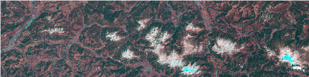
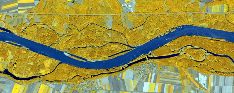
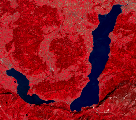
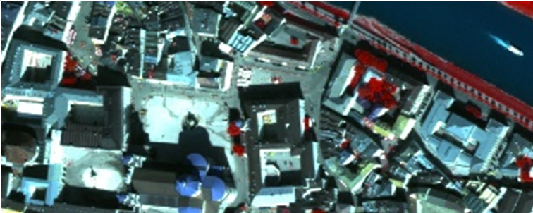
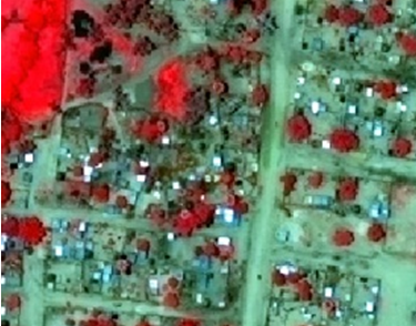
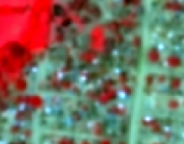
What do the colours mean?
Going back to the starting slide of this unit, we can see a scene which is dominated by red tones.
04.3 (iii) Range adjustments
...

...
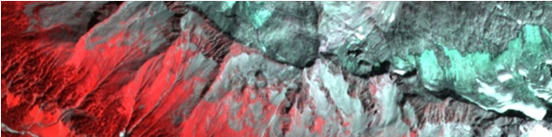
04.3 (iii) Band combinations (incl ArcGIS Pro presets)
Visualising visible and non-visible spectral ranges
...
05 | Spatial referencing
Image Processing & Analysis
05.1 | Spatial referencing
Learning objectives [lesson 5.1]
- Understand the general rationale for spatial referencing and geometric correction
- Learn the purpose of orthorectification and georeferencing
- Understand geodetic and geometric principles as well as the process of (mathematical) transformation and (technical) resampling
05.1 | Spatial referencing
Content and topics [lesson 5.1]
| # | Content | BoK concept |
| i | Rationale of spatial referencing | Spatial referencing |
| ii | Georeferencing vs. geometric correction | * |
| iii | How to obtain real-world coordinates | * |
| iv | Orthorectification via RPC | Orthorectification |
| v | Geodetic principles, projections [recap] | Map projections |
| vi | Transformations & resampling | Coordinate transformations |
05.1 (i) Rationale of spatial referencing
The purpose is to transform image data into a spatial reference frame. The process is carried out according to geodetic principles like the geodetic datum, projections, etc.
There are several ways to 'add' spatial coordinates to an image. This process also compensates for distortion effects that occur during image capturing (applies in particular to ortho-rectification). Usually, images obtained through one of the discussed image portals, are pre-registered or even 'ortho-ready'.

05.1 (ii) Georeferencing vs. geometric correction
Geometric correction is a 'super-concept' comprising georeferencing (external orientation) and ortho-rectification (internal orientation, depending on camera or sensor calibration). The latter is of particular importance for VHR satellite images or air photos.
Resampling is the actual process of re-calculating an image matrix during geometric correction.

05.1 (iii) How to obtain real-world coordinates?
You can obtain real-world coordinates (lat-long [DMS/DD] or metric) from various sources including field visits (GNSS
measurements), Google Maps, Online map portals (e.g. Austrian Map), or any
other co-registered image.

05.1 (iii cont.) How to obtain real-world coordinates?
On-the-fly projection (e.g. in ArcGIS Pro), only if spatial reference information exists.
Image co-registration requires well registered reference image in appropriate resolution

05.1 (iii cont.) How to obtain real-world coordinates?
The geometric quality of an image (pre-registration) depends on the purpose. The pre-registered level 1c / 1g products of Landsat-8 or Sentine-2 are usually sufficient for a typical 'Landsat-like' application case.

05.1 (iv) Orthorectification via RPC
Purpose and procedure VHR Satellite date delivered pre-registered (z.B. UTM-33 / WGS-84) Realized using sensor models (RPC) and differential rectification with DGM Prerequisite: ‘Ortho-Ready‘ products Interpolation of elevation over pixel and re-calculation into image matrix

05.1 (v) Geodetic principles, projections
[add content here]
05.1 (vi) Transformation & resampling
[add content here]
05.2 | GCP collection and referencing
Learning objectives [lesson 5.2]
- Practice the procedure of GCP collection and spatial referencing in the software environmen
- Learn how to assess and improve the quality of the result
05.2 | GCP collection and referencing
Content and topics [lesson 5.2]
| # | Content | BoK concept |
| i | Spatial referencing in ArcGIS Pro | * |
| ii | Image co-registration | Image co-registration |
| iii | Mosaicing | * |
| iv | GCP collection | Ground Control Points (GCP) |
| v | Calculate and assess RMS error | Root mean square error (RMSE) |
06 | Radiometric correction
Image Processing & Analysis
06.1 | Radiometric measurement
Learning objectives [lesson 6.1]
Learning objectives [lesson 6.1]
- Understand the concept of radiometric resolution
- Differentiate the terms reflectance and radiance, and understand the concept of image calibration
06.1 | Radiometric measurement
Content and topics [lesson 6.1]
| # | Content | BoK concept |
| i | Quantisation and radiometric resolution | Radiometric resolution |
| ii | Image calibration (radiance vs. reflectance) | Radiometric correction |
| iii | Principle of atmospheric correction | Atmospheric correction |
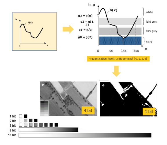
06.1 (i) Quantisation and radiometric resolution
The principle of quantisation is the transformation of a continous brightness range according to a specfied sampling distance, the so-called ground sample distance (GSD). The radiometric resolution corresponds to the number of quantisation levels.
 >
>
06.1 (ii) Image calibration (radiance vs. reflectance)
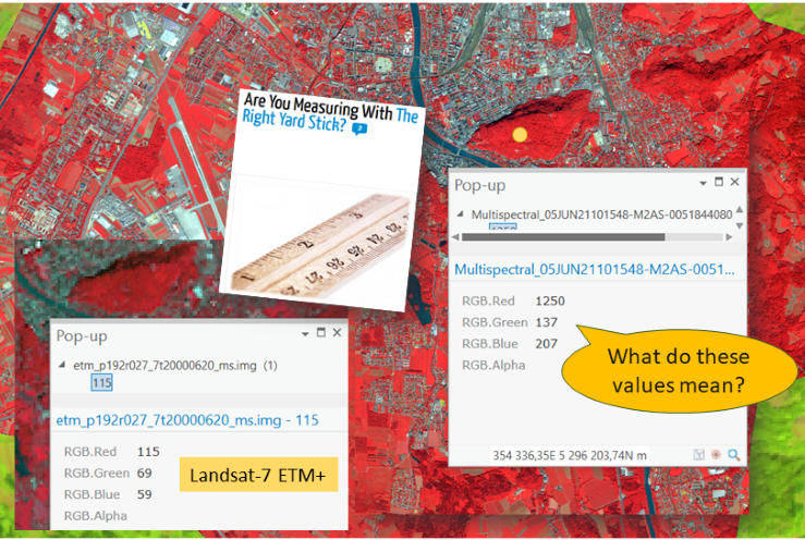
Depending on the radiometric resolution (quantisation levels), image calibration converts digital numbers (DN) into physical units of measurement (spectral radiance)
06.1 (ii cont.) Image calibration (radiance vs. reflectance)
The general workflow of radiometric image enhancement contains radiometric calibration and radiometric correction. Radiometric correction can be separated in atmospheric correction and topographic correction.

06.1 (ii cont.) Image calibration (radiance vs. reflectance)
Image calibration converts digital numbers into radiance at the sensor.

06.1 (iii) Atmospheric correction
Atmospheric correction is a part of radiometric correction compensating for interactions of electromagnetic radiation with gas absorption and aerosol scattering in the atmosphere.

06.2 | Atmospheric correction
Learning objectives [lesson 6.2]
06.2 | Atmospheric correction
Content and topics [lesson 6.2]
| # | Content | BoK concept |
| i | Top-of-atmosphere correction | Converting DN to TOA reflectance |
| ii | Surface correction | * |
06.2 (i) Top-of-atmosphere correction
Top-of-atmosphere (TOA) correction is the most straight-forward radiometric correction based on orbit parameters and celestal constellation. The latter is approximated by the specific sun-earth distance on the particular Iulian day of image acquisition.06.2 (ii) Surface correction
Surface (SURF) correction is a more advanced correction procedure.06.3 | Topographic correction
Learning objectives [lesson 6.3]
- Understand the routine of topographic image correction
- Get an overview of different techniques
06.3 | Topographic correction
Content and topics [lesson 6.3]
| # | Content | BoK concept |
| i | Why topographic correction? | Topographic correction |
| ii | Lambertian correction | * |
| iii | Non-Lambertian correction | * |
06.3 (i) Why topographic correction?
Topographic correction is the process of compensating over- or under-reflectance due to topographic effects and illumination angle. This leads to so-called image 'flattening', because any shading effect etc. disappears.06.3 (ii) Lambertian correction
Lambertian correction ...06.3 (iii) Non-Lambertian correction
Non-Lambertian correction ...07 | Image pre-processing
Image Processing & Analysis
 |
07.1 | Band maths
Learning objectives [lesson 7.1]
Learning objectives [lesson 7.1]
- Understand the purpose of arithmetic band combinations
- Learn how to interpret index values (such as NDVI, NDSI) and their ranges
07.1 | Band maths
Content and topics [lesson 7.1]
| # | Content | BoK concept |
| i | Arithmetic combination of band values | Band maths |
| ii | Spectral ratioing and indices | Spectral indices |
| iii | Vegetation indices | Normalized Difference Vegetation Index (NDVI) |
07.2 | Filtering
Learning objectives [lesson 7.2]
- Understand the principle of contextual focal analysis of images using convolution kernels
- Learn how to apply pre-defined filtering routines for dedicated purposes (sharpening, smoothing, edge detection, etc.)
- Get an idea how filters are used for convolutional neural networks (CNNs)
07.2 | Filtering
Content and topics [lesson 7.2]
| # | Content | BoK concept |
| i | Principle of filtering | * |
| ii | Low-pass vs. high-pass filters | * |
| iii | Weighted filters (Gaussian) | * |
| iv | Directional filters (edge enhancement) | * |
| v | Convolutional neural networks (CNN) | * |
07.3 | Image fusion & PCA
Learning objectives [lesson 7.3]
- Understand the principle of image fusion
- Learn how to perform pan-sharpening techniques (e.g. Gram-Schmid)
07.3 | Image fusion & PCA
Content and topics [lesson 7.3]
| # | Content | BoK concept |
| i | General idea of image fusion | Image fusion |
| ii | Pan-sharpening | Pan-sharpening |
| iii | Computing principle (image) components | PCA |
08 | Image classification
Image Processing & Analysis
08.1 | Multi-spectral classification
Learning objectives [lesson 8.1]
- Understand the purpose of multi-spectral image classification
- Comprehend the difference between supervised and non-supervised classification
- Get to know different classifiers and how they work
08.1 | Multi-spectral classification
Content and topics [lesson 8.1]
| # | Content | BoK concept |
| i | Purpose of digital image classification | Image understanding |
| ii | Spectral characteristics of geographic features [recap] | Spectral signatures |
| iii | Multi-spectral classification | Image classification |
| iv | Supervised vs. non-supervised classification (clustering) | * |
| v | Sample-based vs. knowledge-based classifiers | * |
08.1 (i) Purpose of digital image classification
Why image classification?
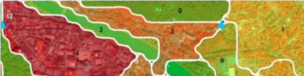
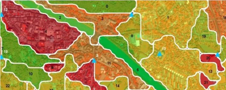
Classification, the conversion of digital numbers into semantic, i.e. meaningful categories (e.g., forest, water, cultivated fields), is the ultimate aim of image analysis. Whenever we look at an image, we instantly ...In pixel-based classification each single pixel is assigned to a given categorical class. This is done according its location in a feature space, but irrespective of its spatial location or surrounding. The general workflow of digital image classification includes:
- ...
- ...
- ...
- ...
- ...
08.1 (ii) Spectral characteristics of geographic features
...08.2 | Supervised classification
Learning objectives [lesson 8.2]
- Learn how to conduct the image classification workflow in ArcGIS Pro
- Practice the collection of samples, the creation of a classification scheme and the selection of a suitable classifier
08.2 | Supervised classification
Content and topics [lesson 8.2]
| # | Content | BoK concept |
| i | Selection of training areas | * |
| ii | Class separability | * |
| iii | Sampling strategies | Sampling strategies |
| iv | Classification schemes | Classification schemes (taxonomies) |
| v | Classifiers in ArcGIS Pro | * |
09 | Quality assessment
Image Processing & Analysis
09.1 | Ground reference & accuracy assessment
Learning objectives [lesson 9.1]
- Understand the meaning of accuracy assessment and how it is performed
- Know what post-process routines exist to improve results
09.1 | Ground reference & accuracy assessment
Content and topics [lesson 9.1]
| # | Content | BoK concept |
| i | Post-processing (majority filtering, reclass, merging classes) | Map algebra (focal analysis) |
| ii | Merging classes and reclass | * |
| iii | Ground validation vs. reference layer | Ground reference |
| iv | Site-specific accuracy assessment | Accuracy assessment |
| v | Error matrix | Error matrix |
09.2 | Product validation
Learning objectives [lesson 9.2]
- Discuss the quality and usabilty of a classification product (and potentially a map generated out of it)
09.2 | Product validation
Content and topics [lesson 9.2]
| # | Content | BoK concept |
| i | Paradoxon of validation | * |
| ii | Usability aspects | * |
| iii | Reproducibility | * |
10 | Publishing results
Image Processing & Analysis
10.1 | Geodata integration
Learning objectives [lesson 10.1]
- Combine image data and with other layers from geodata infrastructures
- Understand the importance of proper spatial referencing
10.1 | Geodata integration
Content and topics [lesson 10.1]
| # | Content | BoK concept |
| i | Data compilation | data integration |
| ii | Harvest OGC compliant sources | integrating data from OGC web services |
| iii | (...) | * |
| iv | (...) | * |
| v | (...) | * |
10.2 | Map making
Learning objectives [lesson 10.2]
- Create a map in the appropriate scale to the image resolution and classification depth
10.2 | Map making
Content and topics [lesson 10.2]
| # | Content | BoK concept |
| i | Create a map | Traditional map making |
| ii | Web mapping | Web map making |
| iii | (...) | * |
| iv | (...) | * |
| v | (...) | * |